For the Instructor
These student materials complement the Modeling Earth Systems Instructor Materials. If you would like your students to have access to the student materials, we suggest you either point them at the Student Version which omits the framing pages with information designed for faculty (and this box). Or you can download these pages in several formats that you can include in your course website or local Learning Managment System. Learn more about using, modifying, and sharing InTeGrate teaching materials.Unit 7 Reading: Global Warming Recorded by Permafrost
by Kirsten Menking, Vassar College
In this week's modeling project, we explore how profiles of temperature versus depth in Arctic permafrost have been used to establish that Earth's high northern latitudes are warming, a phenomenon most likely caused by increased greenhouse gas concentrations in the atmosphere from human activities.
Introduction to Permafrost
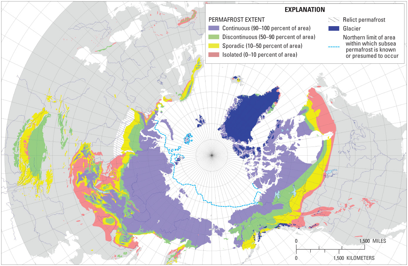
Permafrost, perennially frozen ground that exists at high latitudes and altitudes, covers about a quarter of Earth's land surface (Fig. 1) and forms in locations where mean annual air temperatures (MATs) remain at or below 0 °C for a period of at least two years (Anderson and Anderson, 2010). Where MATs are lower than -6 °C, continuous permafrost forms in which 90–100% of the ground area is frozen (Ritter et al., 2002). In slightly warmer locations (-6 to -1 °C MAT), permafrost may be discontinuous (50–90% frozen ground), sporadic (10-50% frozen ground), or may form in isolated pockets (10% or less frozen ground) in places associated with cold microclimates or where accumulations of moss or peat insulate the underlying soil, preventing it from thawing.
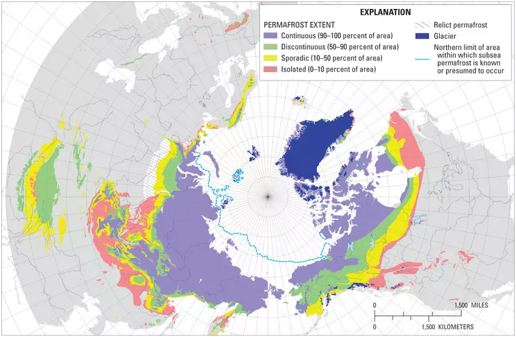 Figure 1: Distribution of permafrost in the northern hemisphere.
![[reuse info]](/images/information_16.png)
Though frozen, permafrost is not the same as glaciers and ice sheets. The latter form when snow piles up on the land surface because summer temperatures are not warm enough to melt the previous cold season's accumulation. Gradually, the weight of the growing snow pile leads to compaction and recrystallization of snowflakes into ice, and once the ice reaches sufficient thickness, it begins to flow under its own weight, forming a glacier.
In many glaciated terrains, accumulation of snow and ice insulates the underlying soil from the cold air above, allowing soil temperatures to remain above freezing and creating thin layers of meltwater at the base of glaciers that permit the ice to slide across the landscape. In contrast, permafrost forms in cold, dry climates where annual snow cover is too thin to act as an insulating blanket and where frigid surface temperatures are able to propagate deeply into the soil. Soil water and groundwater freeze, making frozen ground that may be hundreds of meters thick in regions of continuous permafrost and many meters to tens of meters thick in slightly warmer areas (Fig. 2).
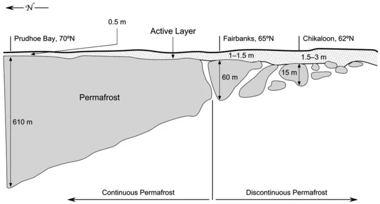 Figure 2: A vertical cross-section shows the extent and thickness of permafrost with latitude.
The thickness the permafrost achieves reflects a balance between the mean annual air temperature in a particular location and geothermal heat coming to the surface from Earth's interior. This geothermal heat is the same heat that drives plate tectonics and consists of a mixture of primordial heat associated with Earth's formation, energy given off by the decay of radioactive elements in the lithosphere, and frictional heat associated with tidal forces. The amount of heat coming to Earth's surface from these sources typically measures between 40 and 90 milliWatts per square meter (Turcotte and Schubert, 1982).
The equilibrium established between MAT at the surface and geothermal heat coming up from below means that a graph of temperature with depth in permafrost shows a negative slope, with temperature lowest at Earth's surface and increasing downward (Fig. 3). Because of the negative slope, the temperature profile crosses over the 0 °C mark at some depth, below which the ground is unfrozen.
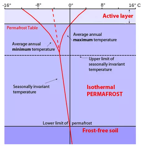 Figure 3: Temperature with depth in permafrost reflects the interaction of heat escaping from Earth's interior with a seasonally fluctuating surface temperature.
![[creative commons]](/images/creativecommons_16.png)
While the MAT required to form permafrost is below freezing, air temperatures vary seasonally near Earth's surface and may occasionally rise above 0 °C. In the summer, the temperature profile in permafrost curls to the right near the surface as warm air temperatures move downward into the soil. In the winter, it curls to the left as exceptionally cold air temperatures chill down the soil. These surface temperature fluctuations affect only a thin layer, however, because it takes time for thermal oscillations at the surface to migrate downward into the ground, and by the time the warmth of summer begins to be felt at depth, the temperature at Earth's surface has again dropped to winter values. At a certain depth, generally not more than a few meters, the geothermal gradient in permafrost ceases to be affected by seasonal variations in MAT and has a constant slope regardless of the time of year (on average, this slope is about 30 °C/km, meaning that for each kilometer of depth increase into Earth, temperature climbs by 30 °C).
In locations where summer air temperatures rise above 0 °C, repeated thawing and refreezing in a thin (a few centimeters to a few meters thick) "active layer" at the surface leads to a number of unusual landforms found only in permafrost regions. These include wedges of massive ground ice, patterned ground (Fig. 4), and ice-cored hills known as pingos (Fig. 5). While we do not have the space to discuss the formation of these landforms in detail, they are generally caused by a segregation of water from soil particles brought about by repeated freeze-thaw activity.
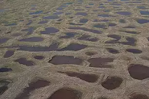 Figure 4: Soil convection caused by an annual cycle of freezing and thawing in permafrost terrains leads to the creation of patterned ground.
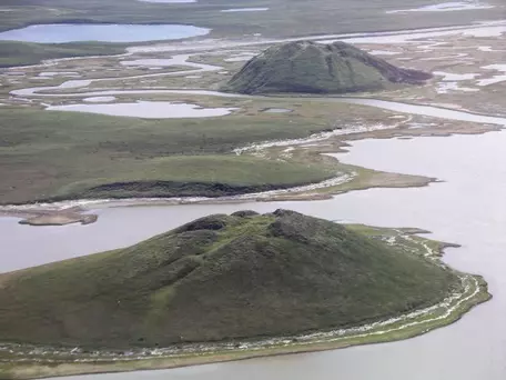 Figure 5: Pingos are ice-cored hills that form in permafrost regions.
The same freeze-thaw cycles that generate permafrost landforms affect human activities and infrastructure. The fact that the ground beneath the active layer remains frozen year-round means that meltwater has nowhere to go in the summer and can pond up on the surface only to freeze again the next winter. Roads built across the tundra collapse when ground ice melts during summer (Fig. 6), limiting the number of roads in the northern half of the state of Alaska.
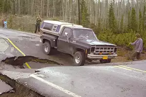 Figure 6: Thawing permafrost leads to differential collapse of the ground, which undermines infrastructure such as roads.
Similarly, the Alaska pipeline that carries crude oil from the state's North Slope to a tanker terminal in the south had to be constructed on stilts in many places to prevent the warm oil from thawing the permafrost, which could lead to differential settling that would damage the pipeline. Other infrastructure is also at risk, and thawing permafrost associated with global warming is projected by the United Nations Environment Program to require the future expenditure of several billion dollars in maintenance costs in Alaska alone (http://epic.awi.de/33086/1/permafrost.pdf). Add in Russia, Canada, Norway, and other nations with substantial permafrost coverage, and the costs of Arctic warming are projected to climb even higher.
Permafrost as a Recorder of Climatic Change
In the mid-1980s, climate science was still in its infancy and evidence for global warming had only recently begun to be collected. While climate models predicted that global temperatures should rise in response to increased fossil fuel combustion and resulting greenhouse gas production, weather records were still relatively short and showed a lot of variability over time, making it difficult to determine whether warming trends were related to human activities or to natural cycles in the climate system. Also problematic was the fact that few weather records existed for the Arctic.
Geoscientists Arthur Lachenbruch and Vaughn Marshall realized that rather than looking at weather records, they could use inflections in the geothermal gradient of permafrost to search for evidence of climatic change. Their reasoning was thus: if mean annual temperature at some locality were to remain constant over a long period of time, the geothermal gradient in that spot should be fairly uniform with depth. However, if the MAT were to change, either to become warmer or to become colder, the gradient would have to adjust itself to the new surface temperature. Because the movement of heat through a medium is not instantaneous, but rather takes time, the surface layers of soil and rock would respond to the change well before the deeper layers. This variation in the time of response would create a "kink" in the geothermal gradient with depth analogous to the kink produced by seasonal oscillations in surface temperature.
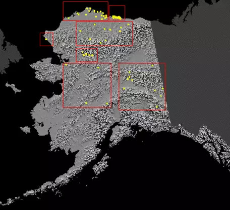 Figure 7: This map of Alaska shows the location of boreholes where permafrost temperatures have been measured over the past several decades.
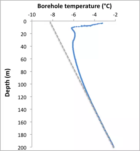 Figure 8: Borehole temperatures from the Awuna site in Alaska (blue dots) show a pronounced kink in the geothermal gradient consistent with a recent (last few decades) warming of >2 °C. The dashed gray line shows what the geothermal gradient would look like in the absence of this warming. Data available at http://gec.cr.usgs.gov/data/bht_alaska/sites/AWUN/AWUN_84JUL29.log.
To determine whether Arctic permafrost showed evidence for recent warming, Lachenbruch and Marshall (1986) dropped thermistors (a type of thermometer) into exploratory boreholes drilled in Alaska's North Slope oil field area (Fig. 7) by companies prospecting for new oil and measured temperature at many different depths. In general, the thermistors registered anomalously high temperatures well below the depth where seasonal fluctuations are felt (Fig. 8). While Lachenbruch and Marshall did not pass judgment on whether the observed warming was due to human activities, they did note that a 2–4 °C rise in near-surface permafrost temperature over the last several decades was consistent with model predictions of global warming brought about by fossil fuel combustion. In the years since their work was published, additional studies have confirmed their results and shown that borehole temperatures faithfully record changes in Earth's surface temperature over time.
Heat Flow in Permafrost
The reason why permafrost is such an effective recorder of temperature changes at Earth's surface is because the water it contains is frozen and does not circulate. This means that the only way for heat to be transmitted through the ground is via conduction, the process by which kinetic energy from fast-moving molecules is transferred to slower-moving molecules through collision. If you have spent any time in the kitchen, you have already become quite familiar with conduction because it is the mechanism by which heat is transferred from a burner on a stovetop into a saucepan or skillet. Transfer of heat by conduction can be described mathematically by Fourier's Law, which relates the flux of heat through a substance (`Q`) to the temperature difference across it (` (delT)/(delz)`) and to its thermal conductivity (`k`), an inherent material property that describes how readily a substance transmits heat:
` Q=-k(delT)/(delz)`
In the case of heat flow in permafrost, the ` (delT)/(delz)` in Fourier's law is the geothermal gradient, and `k` is the thermal conductivity of the frozen soil, a mixture of mineral particles, organic matter, and ice. Note that Fourier's Law has a minus sign in it. The reason for this is that heat flows out of Earth's interior toward its surface, but temperature in the earth increases downward, into Earth.
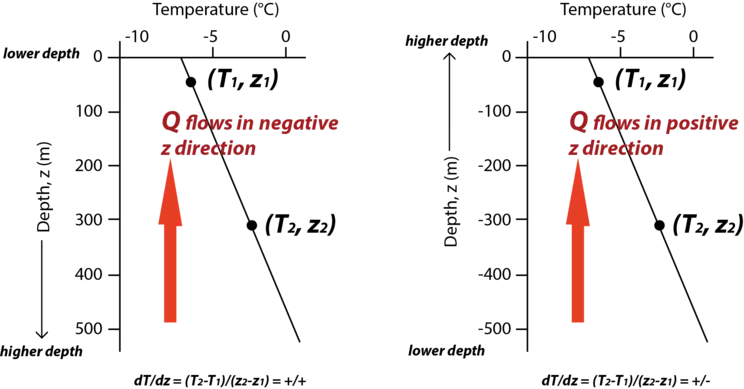 Figure 9: Two ways of visualizing the flow of heat (red arrow) from Earth's interior. Note that on the left side we show depth increasing downward into Earth, whereas on the right side, depth is increasing upward, out of Earth.
If we set up a coordinate system that has 0 m depth at Earth's surface and that increases in depth into Earth (Fig. 9 - left side), then measuring ` (delT)/(delz)` gives a positive change in temperature with depth since a cooler temperature near Earth's surface is subtracted from a warmer temperature at depth (a net positive value) in order to calculate ` delT` while a lower depth near Earth's surface is subtracted from a higher depth in the interior (a net positive value) to calculate ` delz`. In this case, the minus sign is used to achieve the correct sign for the heat flow value, which is in the opposite direction of the increase in depth. If this seems confusing, you can also flip the coordinate system such that the scale starts at 0 m depth at Earth's surface and then decreases downward into Earth (Fig. 9 - right side). In this scenario, a cooler temperature near Earth's surface is subtracted from a warmer temperature at depth (a net positive value) in order to calculate ` delT` while a higher (less negative) depth near Earth's surface is subtracted from a lower (more negative) depth in the interior (a net negative value) to calculate ` delz`. Since Q is flowing in the same direction as z is increasing, a negative sign must be multiplied by the resulting negative value of ` (delT)/(delz)` in order to ensure that Q is positive upward.
We are going to create a numerical model of heat flow in permafrost to see if we can replicate some of Lachenbruch and Marshall's findings. Before doing so, we will discuss the problem of heat flow in Earth's crust more generally to help you develop an understanding of why the geothermal gradient changes in response to a temperature change at the surface.
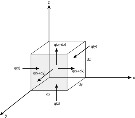 Figure 10: A small piece of crust through which heat energy (q) is flowing in the x, y, and z dimensions.
To begin, let us consider a small piece of rock sitting at some depth within Earth's crust (Fig. 10), and let us assume that this piece has dimensions dx, dy, and dz. The total amount of heat energy contained in this piece of rock at any given time (E(t)) depends on its mass (m), its specific heat (c), and its temperature (T). This can be represented mathematically as:
` E(t)=mcT `
Specific heat is a measure of the amount of heat necessary to raise the temperature of a unit mass of a material by 1 °C and typically has units such as Joules/(kg °C). When multiplied by the mass (typically in kg), and the temperature (°C), the specific heat returns a value of energy (joules) for E(t).
Now recall that mass can be determined by multiplying density (` rho `) by volume (dx*dy*dz). For our small piece of rock then,
` E(t)=rhodxdydzcT `
which can be rearranged to
` E(t)=rhocTdxdydz `
At some future time (t + dt), the flow of heat into and out of our small piece of rock will change the amount of energy the piece contains to E(t+dt). We use a Taylor series expansion to determine the value for E(t+dt):
` E(t+dt)=rhocTdxdydz + (del(rhocTdxdydz))/(delt)dt + "higher order terms" `
The values of the higher-order terms are generally so small compared to the first two parts of the right-hand side of the equation as to be negligible. To see how much the energy contained within the piece of rock has changed over time, we subtract E(t) from E(t+dt), which leaves:
` (delE(t))/(delt)dt=(del(rhocT))/(delt)dxdydzdt ` when we ignore the higher-order terms. The dxdydz part of the equation can be removed from `(del(rhocTdxdydz))/(delt)dt` because the volume of the piece of rock does not change with time.
Now let us look at the heat flowing through the small piece of rock. Heat can move into and out of the piece in all three dimensions, x, y, and z. If the amount of energy in the piece changes over time, then the amount of energy entering the piece must be different from the amount of energy leaving the piece of rock. We keep track of the amounts entering and leaving for all three dimensions with the equations:
` q_x(x) - q_x(x+dx) = -(delq_x)/(delx)dxdydzdt ` (flux of heat in the x-dimension)
` q_y(y) - q_y(y+dy) = -(delq_y)/(dely)dxdydzdt ` (flux of heat in the y-dimension)
` q_z(z) - q_z(z+dz) = -(delq_z)/(delz)dxdydzdt ` (flux of heat in the z-dimension)
Note that in each of these equations, the amount of energy flowing out of the piece is subtracted from the amount of energy entering the piece. For example, in the x-direction, the amount of energy flowing out of the piece, ` q_x(x+dx)`, is subtracted from the amount of energy flowing into the piece, ` q_x(x)`, and the distance between where the energy flows in and where it flows out is represented by dx.
If we now recognize that the change in the amount of heat energy in the piece of rock with time is due to changes in the amount of heat entering and leaving the piece of rock over space, we can come up with the following expression:
` (del(rhocT))/(delt)dxdydzdt = -(delq_x)/(delx)dxdydzdt-(delq_y)/(dely)dxdydzdt-(delq_z)/(delz)dxdydzdt `
All terms in this equation contain dxdydzdt, which allows us to remove it from both sides of the equation to leave:
` (del(rhocT))/(delt) = -(delq_x)/(delx)-(delq_y)/(dely)-(delq_z)/(delz) `
We will now make a simplifying assumption that the amount of heat flowing into and out of the piece of rock varies only in the vertical (z) dimension. In other words, we will assume that ` q_y(y) - q_y(y+dy) = 0` and that ` q_x(x) - q_x(x+dx) = 0`. This is probably justifiable since the amount of heat traveling vertically from Earth's interior to the surface is more likely to vary, given the vast temperature difference between Earth's interior and the surface, than the amount of heat flowing in either of the two horizontal dimensions. With this simplifying assumption,
` (del(rhocT))/(delt) = -(delq_z)/(delz) `
Rearranging, we get:
` (delT)/(delt) = -1/(rhoc)(delq_z)/(delz) `
Earlier we introduced Fourier's law of heat conduction, which stated that ` Q=-k(delT)/(delz)`. Recasting that equation in the symbols we're using at present,
` q_z=-k(delT)/(delz)`
If we now substitute this expression into the previous equation, we get:
` (delT)/(delt) = -1/(rhoc)(del (-kdelT)/(delz))/(delz) `
This simplifies to:
` (delT)/(delt) = k/(rhoc)(del \ ^2T)/(delz ^2) `
Let,
` K= k/(rhoc)`, where ` K` is known as the "thermal diffusivity."
Then,
` (delT)/(delt) = K(del \ ^2T)/(delz ^2) `, which is known as the thermal diffusion equation. This equation has an analytical solution that requires quite a bit of calculus to acquire. Fortunately, our numerical model does not require the analytical solution as it will be using the finite difference method to approximate the solution, using Fourier's Law only to keep track of the flow of heat from one level in Earth's crust to another. Still, it is worth looking at this equation and thinking about what it means. When translated into English, the symbols tell us that the change in temperature over time in our small piece of rock (` (delT)/(delt)`) is related to the second derivative of the temperature with depth (` (del \ ^2T)/(delz ^2) `).
What does this second derivative mean? We can understand it better if we look at a similar equation that describes the evolution of topography over time in response to erosion and deposition. Consider a hilly landscape in two dimensions, x and z (top graph in Fig. 11).
 Figure 11: A hilly landscape z(x) has slopes of ` dz/dx ` and changes in slope (curvature) of ` (d \ ^2z)/(dx^2) `.
In this landscape, erosion occurs at the hillcrests and deposition occurs in the valleys. As a result, the elevation of the landscape changes with time, which can be described mathematically with the topographic diffusion equation:
` (delz)/(delt) = K(del \ ^2z)/(delx^2) `
Let us think about what this equation is saying. ` (delz)/(delt) ` is the change in elevation with time. This value depends on the curvature ( ` (del \ ^2z)/(delx^2) `) of the landscape and the diffusivity (K). Where the curvature is strongly negative, as it is at the crest of a hill, then the change in elevation with time is also negative, meaning that the hillcrest erodes downward (Fig. 12). Where the curvature is strongly positive, as it is in a valley, then the change in elevation with time is also positive, and the eroded sediment from the hillcrest fills in the valley.
 Figure 12: The diffusion equation for topography creates erosion on hillcrests and deposition in valleys.
The thermal diffusion equation works in an analogous way, but instead of looking at how elevation changes with distance, we are instead looking at how temperature changes with distance (depth). Just as a high positive curvature in the topographic diffusion equation leads to deposition and an increase in elevation with time, where there is high positive curvature in the thermal diffusion equation, the temperature rises over time. Where there is high negative curvature, the opposite is true and temperature declines. Consider the following example: after millennia of constant temperature, air temperature suddenly rises, leading to a kink in the geothermal gradient (Fig. 13). The high positive curvature associated with the kink means that thermal diffusion will gradually smooth out the profile and will eventually cause all of it to shift to the right (see the dashed lines in Fig. 13).
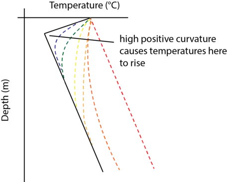 Figure 13: Warming at Earth's surface leads to a kink in the geothermal gradient (black line) that smoothes out over time due to thermal diffusion. Dashed lines represent different time slices in the evolution of the geothermal gradient, with the blue line representing the earliest response to the thermal perturbation and the red line representing the final equilibrium gradient for the new, warmer surface temperature.
In the STELLA model we create today, we explore the impacts of a variety of different climate change scenarios (step change, surface temperature oscillations of different frequencies) on the geothermal gradient and compare our results to the borehole data shown in Figure 8. We will use a simplified model that ignores the impact of insulating materials, such as layers of snow or peat, on heat conduction and that also ignores the possibility of ice melt during the warmer summer months. These factors can affect the movement of heat and add complexity to the response of permafrost to changes in air temperature. Still, our simple model will allow us to learn a lot about how climate change can affect the geothermal gradient.
References
Anderson, R.S., and Anderson, S.P., 2010, Geomorphology: The Mechanics and Chemistry of Landscapes, New York: Cambridge University Press, Chapter 9, Periglacial processes and forms.
Lachenbruch, A.H., and Marshall, B.V., 1986, "Changing Climate: Geothermal Evidence from Permafrost in the Alaskan Arctic," Science, v. 234, p. 689–696.
Ritter, D.F., Kochel, R.C., and Miller, J.R., 2002, Process Geomorphology, 4th edition, New York: McGraw-Hill, Chapter 11, Periglacial Processes and Landforms.
Turcotte, D.L., and Schubert, G., 1982, Geodynamics: Applications of Continuum Physics to Geological Problems, New York: John Wiley and Sons, Chapter 4, Heat Transfer.


