For the Instructor
These student materials complement the Modeling Earth Systems Instructor Materials. If you would like your students to have access to the student materials, we suggest you either point them at the Student Version which omits the framing pages with information designed for faculty (and this box). Or you can download these pages in several formats that you can include in your course website or local Learning Managment System. Learn more about using, modifying, and sharing InTeGrate teaching materials.Unit 5 Reading: Ice Sheet Modeling
by David Bice, The Pennsylvania State University
In this exercise, we will do some experiments with a simple ice sheet model based on a classic paper by Johannes Weertman from 1976. Our goals are to understand some basic things about how these ice sheets grow and shrink, and how they can respond to insolation variations caused by orbital changes of Earth relative to the sun.
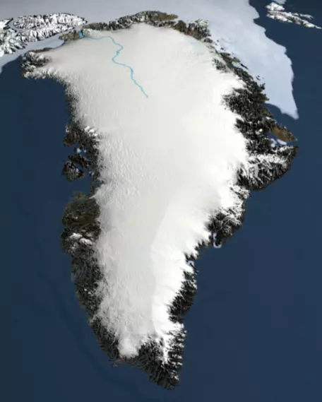 Figure 1. The Greenland Ice Sheet is approximately 2500 km N-S and about 1300 km E-W near its middle. The ice in the center is about 3000 m thick, with a total volume of 2.6e6 km3, which represents a potential sea level rise of about 6.5 m.
 ![[reuse info]](/images/information_16.png)
Large continental ice sheets such as Greenland (Fig. 1) are important components of the global climate system — they play a critical role in altering the planetary albedo, which is connected to a potent positive feedback mechanism, and also in controlling global sea level.
The growth and decline of large ice sheets has been one of the dominant features of the Pleistocene ice age (Fig. 2), and their current decline is of great importance to the rising global sea level. The timing of the ice ages and intervening warmer periods are largely controlled by orbital changes, and one of the goals of this modeling exercise is to see how this works — how the ice sheet system responds to the orbital changes.
To develop our model of an ice sheet, we have to start with a few basics of how ice forms and flows. Glacial ice begins as snowfall that accumulates over the years. As it gets buried under more snow, the snow crystals undergo a kind of metamorphism, eventually turning into solid ice. Ice, as a naturally occurring polycrystalline solid, is really a kind of rock, but unlike most other rocks, ice can actually flow at the surface without melting. This solid-state flow is quite fast relative to other geologic processes, enabling glaciers to be very dynamic features of the surface.
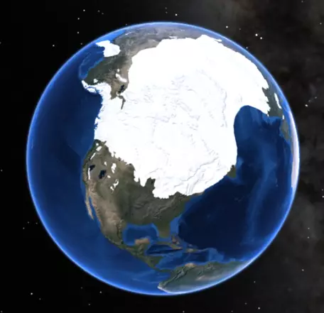 Figure 2. Reconstruction of the ice extent during the last glacial maximum, around 20 kyr BP.
It is common to assume that ice behaves as a deformable plastic material, which means that there is a critical shear stress, τ0, below which no strain (deformation or flow) will occur, and above which, the strain is limitless. Stress is simply a force acting on an area, and shear stress is a force applied parallel to a surface as opposed to a force applied perpendicular to a surface, which is called a normal stress. We talk about stresses rather than forces, since stresses are what can cause materials to deform (whether by flow or by fracture). The shear stress at the base of a pile of ice (Fig. 3) is a function of the surface slope, the thickness, gravity, and density:
` tau_b = rhoghsinalpha ` Eqn. 1
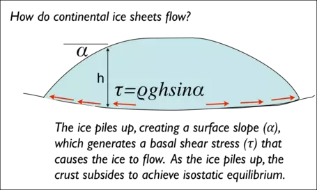 Figure 3. Schematic slice through an ice sheet, showing how the surface slope, ` alpha`, and the thickness, h, along with gravity and density, ` rho`, dictate the shear stress that drives the flow of ice.
 ![[creative commons]](/images/creativecommons_16.png)
Here, ` rho ` is the density of ice (typically 920 kg/m3), g is the acceleration due to gravity, h is the height of the ice, and ` alpha ` is the surface slope angle. When ` tau_b ` is greater than or equal to ` tau_0 `, then the ice will flow. This equation tells us that where the thickness of the ice is greater, the slope can be smaller and still achieve the critical shear stress. Where the ice is thinner, a higher surface slope is needed to get the critical shear stress. Considering that the height or thickness of the ice must taper to 0 at the edge, you can see that the slope of the glacier has to be greatest right at the edge (which is illustrated in a schematic way in Fig. 3).
If the slope is too low, the basal shear stress will not match the critical shear stress ` tau_0 `, but as snow piles up, creating more ice, the thickness (h) will increase until ` tau_0 ` is reached, at which point, flow will begin. As flow begins, the slope will decrease; this causes the basal shear stress to drop below ` tau_0 ` and flow will stop, but then snow piles up again and ` tau_0 ` is met. The result of this is that the glacier evolves to the point where the basal shear stress all along its base hovers right around the critical shear stress ` tau_0 ` and a steady state condition occurs. The result of this is that a glacier has an equilibrium profile, which can be obtained from the equation for the basal shear stress, rewritten as follows:
` tau_0 = rhoghsinalpha = rhogh(-(dh)/(dx)) ` Eqn. 2
Here, ` (dh)/(dx) ` is the change in height divided by the change in horizontal distance, essentially the slope of the glacier's surface. The goal here is to find an expression for the equilibrium profile — how h varies as a function of horizontal position, x. The first step is to rearrange Eqn. 2 to get:
` hdh = -tau_0/(rhog)dx ` Eqn. 3
Next, we integrate both sides:
` 1/2h^2 = -tau_0/(rhog)x + C ` Eqn. 4
Here, C is the combined constants of integration from both sides. To figure out what C is, we need to have some kind of boundary condition. In this case, we know that at the edge of the glacier, which we will call L, the height of the glacier, h, is 0; in other words, at x=L, h=0. We plug this into Eqn. 4 to get:
` 1/(2)0^2 = -tau_0/(rhog)L + C `, so `C = tau_0/(rhog)L ` Eqn. 5
Then, we plug this expression for C into Eqn. 4, which gives:
` 1/2h^2 = -tau_0/(rhog)x + tau_0/(rhog)L ` Eqn. 6
This can be rearranged to give us:
` h^2 = (2tau_0)/(rhog)(L - x), or h(x) = sqrt((2tau_0)/(rhog)(L - |x|)) ` Eqn. 7
This final equation gives us a description of how the height of the glacier, h, changes as a function of distance, x, from the center of the ice sheet. Here, x = 0 is the center of the ice sheet, and by using the absolute value of x, we end up with a symmetrical profile for the glacier. To show how this works, imagine that we have an ice sheet with a length, L, of 3000 km (this is about the size of the Laurentide Ice Sheet that covered a large portion of North America in the last ice age), a critical shear stress of 75 kPa (75,000 Pa; Pa = Pascal, a unit of stress in N/m2), and a density, ` rho `, of 920 kg/m3. Plugging these numbers into Eqn. 7, we get the thickness at the center of the glacier (where x = 0):
` h(x = 0) = sqrt((2 * 75e3)/(920 * 9.8)(3e6 - 0)) ~~ 7000 ` m Eqn. 8
We make one slight simplification of Eqn. 7 as follows:
` h(x) = sqrt(lambda(L - |x|)) ` where ` lambda = (2tau_0)/(rhog) ` Eqn. 9
Weertman says that typical values for ` lambda ` are 8 – 15 (the units in meters). If you integrate Eqn. 9 from x = -L to x = L, you get the cross-sectional area of the glacier, and you can also flip this around to get the length from the cross-sectional area:
` A_x = 4/3 lambda^(1/2)L^(3/2) ` and conversely, ` L = ((3/4A_x)^2/lambda)^(1/3) ` Eqn. 10
Figure 4 shows what the shape of the glacier looks like, at two different times, with different cross-sectional areas:
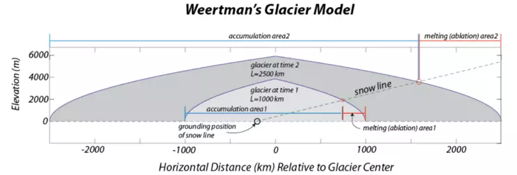 Figure 4. Cross-section through the model ice sheet, showing its profile at two different times, along with the intersection points (circled) of the snow line (dashed) and the glacier surface. In this model, the snow line rises to the right, which means that the right side is warmer (south, if this is the Laurentide Ice Sheet). The position of the snow line on the glacier surface, xs, then determines the accumulation and ablation areas of the ice sheet. Also shown is the grounding line position of the snow line, which can move back and forth due to climate changes. The ice sheet grows until the accumulation area multiplied by the accumulation rate (mass added) equals the ablation area times the ablation rate (mass lost).
Also shown in this diagram is the snow line, which separates colder areas where snow will accumulate to form ice from warmer regions where the melting exceeds snowfall, and the glacier will experience a loss of ice. The snow line slopes gently up to the right toward the warmer, equatorward side of the diagram. Where this snow line intersects the surface of the glacier (red circles in Fig. 4), we divide the glacier into its accumulation zone and its melting zone. The grounding position (black circle in Fig. 4) marks the place where the snow line intersects an elevation of zero. In Weertman's model, it is assumed that the right side of the ice sheet in Figure 4 is to the south; the left is the north. Weertman did not discuss the northern half of the ice sheet, but we presume that iceberg calving on the northern edge balances the accumulation. Thus, the northern half of the ice sheet is a "slave" to the location of the ice divide, which in turn is controlled by climate.
The model starts with an initial glacier length, and from that, we can calculate the profile of the glacier and its cross-sectional area. Once we have the profile, we can find the intersection with the snow line, which allows us to separate the glacier into the regions above the snow line, where accumulation can occur, and below the snow line, where melting will occur. We get the point where the snow line intersects the glacier surface by setting the equation for the snow line,
` h_s = S(x - x_g) ` Eqn. 11
in which S is the slope of the snow line, and xg is the grounding line position, equal to the equation for the shape of the ice surface,
` h_i = sqrt(lambda(L - |x|)) ` Eqn. 9
This leads to a quadratic equation that gives us the x position of the point where hi=hs.
` x_s = (-b + sqrt(b^2 - 4ac))/(2a) ` Eqn. 12
where ` a = S^2 `, ` b = lambda - 2x_(g)S^2 `, and ` c = S^2x_g^2 - lambdaL `
Once we have the snow line, we can calculate the change in the cross sectional area of the glacier as follows:
` (dA_x)/(dt) = L_(ac)nu_(ac) - L_(ab)nu_(ab) ` Eqn. 13
This is a simple differential equation that tells us how the cross-sectional area (Ax) changes over time — if it is positive, the glacier will grow, if negative, then the glacier shrinks, and if it has a value of 0, the glacier is in a steady state condition. Here, Lac is the length over which accumulation occurs (Lac = L + xs), and Lab is the length over which melting or ablation occurs (Lab = L - xs). These lengths are multiplied by their corresponding rates, ` nu_(ac) ` and ` nu_(ab) `, and then summed to give the change in cross-sectional (Ax) over a given interval of time. The balance of accumulation and ablation — the sign of equation 13 — then determines if the glacier will shrink or grow; in either case, we assume that it maintains the equilibrium profile. In the model, the accumulation rate (` nu_(ac) `) and ablation rate (` nu_(ab) `) are related by a parameter called epsilon:
` epsilon = nu_(ac)/nu_(ab) ` Eqn. 14
This parameter epsilon is useful because it also helps us understand something about the steady state condition, which is when equation 13 is equal to 0. If we set that equation to 0 and then rearrange things, we get:
`0 = L_(ac)nu_(ac) - L_(ab)nu_(ab) ` so,
`L_(ac)nu_(ac) = L_(ab)nu_(ab) ` or,
` nu_(ac)/nu_(ab) = L_(ab)/L_(ac) = epsilon ` Eqn. 15
In other words, when the ratio of the ablation length to the accumulation length is the same as epsilon (the ratio of ablation rate to accumulation rate), the ice sheet will be in a steady state — there will be no change in the cross-sectional area.
If warming occurs, the grounding line moves to the left (-x is considered to be toward the north), whereas cooling moves it to the south (right in the diagram). Based on observations of the present, Weertman calculated that the grounding position of the snowline changes by 17.7 km for every W/m2 of mean summer insolation change.
When Weertman wrote his paper, geoscientists were actively searching for ways to test the astronomical theory of climate change, attributed to Milankovitch, who showed that orbital variations (on timescales of tens to hundreds of kyr) should lead to seasonal changes in insolation that could explain the Pleistocene glacial-interglacial cycles. There are some orbital configurations that lead to relatively mild summers, which prevents all the previous winter's snow from melting, thus allowing for the buildup and growth of ice sheets. Once the ice sheets begin to grow, the ice-albedo feedback mechanism kicks in and significant cooling results. In fact, the same year as Weertman's paper, Hays et al. (1976) showed oxygen isotope evidence from marine sediment cores that the Pleistocene climate changes were controlled by these orbital variations. We can think of Weertman's paper as an examination of whether this idea makes sense in terms of the physics and dynamics of ice sheets. Before discussing how these orbital changes are implemented into the model, it is a good idea to briefly review what these orbital variations are.
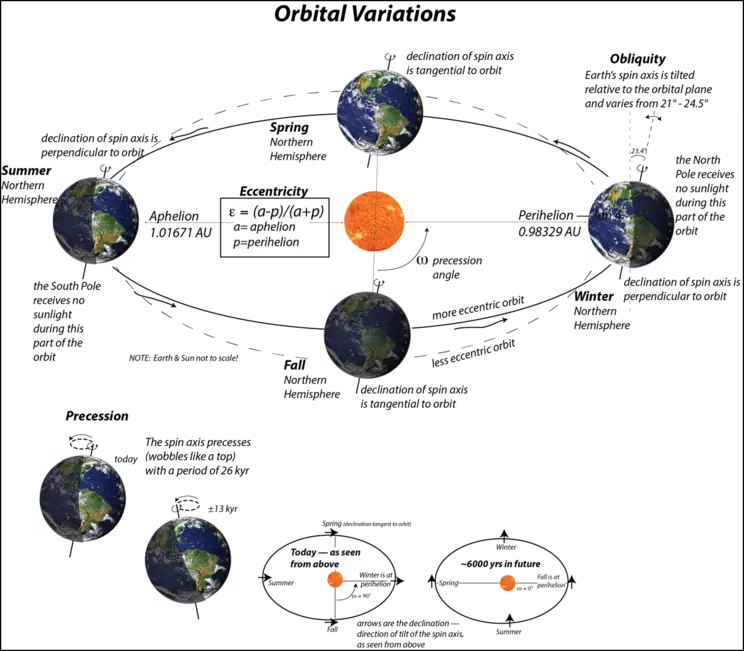 Figure 5. Orbital variations of Earth include the eccentricity of the orbital path, the obliquity or tilt angle of the spin axis, and the precession of the spin axis. Not shown here is the slow rotation of the orbital path around the sun.
Earth's orbit around the sun changes in three main ways (Fig. 5). Our path around the sun varies from being more circular to more elliptical due to the gravitational effects of Jupiter, Saturn, and to a lesser extent, Mars. The deviation from a perfect circle is called the eccentricity of the orbit, and this changes in a complicated way as the sum of three cycles, with periods of 95, 125, and ~400 kyr. As the eccentricity gets bigger, there is a greater difference between perihelion (the shortest Earth-sun distance) and aphelion (the greatest Earth-sun distance). The tilt angle, or obliquity, of our spin axis with respect to the orbital plane also changes from 22° to 24.5° away from perpendicular, with a cycle of 41 kyr. The tilt angle is important in accentuating seasonal differences — a higher tilt angle means a greater difference between summer and winter — and it affects the polar regions more than the equatorial regions. The third variation in our orbit arises from the precession of the spin axis — it wobbles just like a top due to torque applied by the sun and moon, which has an effect due to the equatorial bulge of Earth (equatorial diameter is about 45 km greater than the polar diameter). The precession of the spin axis changes the position in the orbit when we have winter, spring, summer, and fall. Currently, our winter solstice occurs very close to the perihelion position, so the precession angle (` omega ` in Fig. 5) is about 103°. The period of the precession is 26 kyr, but this interacts with the slow rotation of our orbital path around the sun to produce periods of 19–24 kyr.
If our orbit were a perfect circle, the precession of the spin axis would not have any real effect on insolation, but, when combined with the eccentricity, precession does have a big effect. For instance, in our present configuration, summer occurs near the aphelion position, and we have a relatively long, cool summer (long because the velocity of Earth around the orbit slows down as it gets farther from the sun). A cool summer in the polar regions means that there is a chance that all of the previous winter's snow might not melt, which could then lead to the buildup of glacial ice. Right now, the eccentricity is quite low, so the summers are not that cool, but with a higher eccentricity, our present configuration could lead to the growth of a large polar ice sheet and a new glacial age.
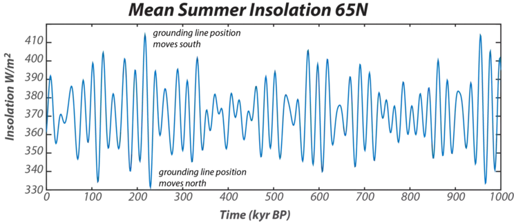 Figure 6. Mean summer insolation for 65°N shows the combined effects of eccentricity, obliquity, and precession over the past 100 kyr.
These orbital variations combine to produce significant variations in the insolation received at different places on Earth (Fig. 6), but these variations in the Northern and Southern Hemispheres are out of phase with each other, so there is no net change in the insolation received by the whole planet. But, our climate system has sensitive spots where even a slight change can trigger a feedback mechanism that amplifies the initial change. The Arctic region is one of these sensitive spots because the abundant land mass in the Northern Hemisphere makes it possible to grow a very large ice sheet, and the biggest part of the oceanic thermohaline circulation can be turned on or off by changes in the area around Iceland. Indeed, it turns out that oxygen isotope records from ice cores (temperature proxy) and marine sediments (proxy for ice volume and temperature) both match the summer insolation curve for 45°N to 65°N (the insolation curves are very similar for this latitude range).
In our ice sheet model, the summer insolation will control the position where the snow line meets the ground (we will call this the grounding line); this in turn will control the position of the snow line on the ice sheet, which in turn controls whether the ice sheet grows or shrinks. Weertman estimated that the grounding line moves 17.7 km for every W/m2 change in the summer insolation, and given a range of about 110 W/m2, this translates into a grounding line movement of over 1900 km, around 17° of latitude. So, we might expect this variation in insolation to have a significant impact on the dynamics of the ice sheet. Why do we say might expect rather than definitely expect? The reason is that it depends on the response time of the ice sheet in comparison with the frequency of the insolation variation — if the response time of the ice sheet is very long relative to the insolation change, then the insolation change will not have much of an impact.
Consider this simple illustration of the concept. We take a very simple climate model of Earth based on an energy balance where the insolation from the sun is balanced by the emission of infrared radiation, following the Stefan-Boltzmann Law (Fig. 7). This model is set up to be in a steady state at a temperature of 288 K, which is 15°C. Given the depth of the ocean, the heat capacity of water, and the density of water, this system has a response time of about five years.
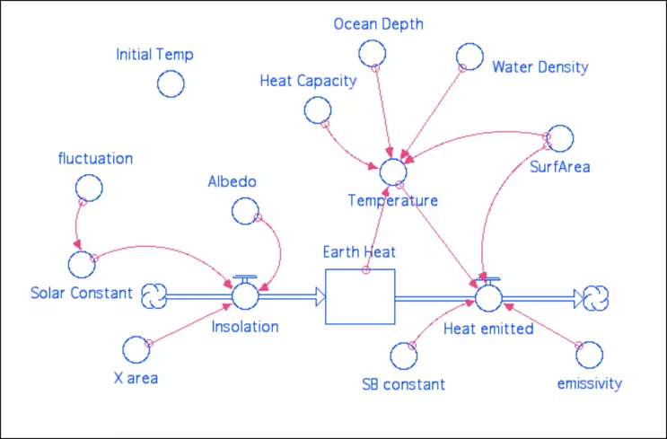 Figure 7. A simple planetary energy balance climate model of Earth, with a fluctuating solar constant to illustrate how a system's response to a perturbation is dependent on the period or frequency of the perturbation relative to the natural response time of the system.
We perturb this steady state by adding a fluctuation of ±10 W/m2 to the solar constant, which is normally 1370 W/m2. If we just add 10 W/m2 to the solar constant and let the climate get into a new steady state, it will warm by 0.5°, but let us consider what happens when the change to the solar constant is a sinusoidal function with a period that varies from one model run to the next. In Figure 8, the period varies over the course of five model runs from 0.2 to 1.0 to 5 to 10 to 20 yrs — the first two are shorter than the response time for the system (5 years), while the last two are greater than the response time. In all cases, the magnitude of the change is the same — ±10 W/m2.
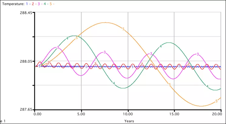 Figure 8. Temperature changes experienced by the climate model of Fig. 7 in response to fluctuations with an amplitude of 10 W/m2 and varying periods. Curve 1 has a period of 0.2 yrs; curve 2: 1 yr; curve 3: 5 yrs; curve 4: 10 yrs; curve 5: 20 yrs. The natural response time of the climate system is about five years, and fluctuations in the solar constant with a period of less than five years have little impact on the temperature, while periods greater than five years have a more significant impact.
As we can see, the magnitude of the resulting temperature change is strongly affected by the period of the fluctuation. When the fluctuation occurs at a high frequency, the system cannot keep up with the fluctuation — before the climate can warm in response to the higher solar constant, the solar constant has begun to decrease, and this brings the warming to a halt well before it reaches the 0.5° value that would normally result from an increase of 10 W/m2. In other words, the system does not have enough time to respond to the solar fluctuations. In contrast, when the fluctuation occurs at a low frequency (long period), the system does a better job of keeping up with the fluctuation.
The point of this digression is just to help you see that the question of how much the ice sheet will change due to the variations in insolation depends on the natural response time of the ice sheet, which itself is a function of the mathematics of the model. It is tricky to derive this response time, but once we make the model, we can easily see what the response time is.
One final note is that Weertman's model is for a continental ice sheet, and there are other, more complex models for marine ice sheets. Marine ice sheets behave somewhat differently, but they are also important to the climate system. For instance, some models of marine ice sheets show complex internal variability that could lead to the kind of massive iceberg discharge events (the Heinrich events) observed in the Pleistocene — these changes are not linked to orbitally-induced changes in the snow line grounding position.
Additional Reading:
Weertman, J., 1976, "Milankovitch solar radiation variations and ice age sizes of ice sheets," Nature, v. 261, p. 17–20.
Hays, J.D., Imbrie, J., and Shackleton, N.J., 1976, "Variations in Earth's Orbit: Pacemaker of the Ice Ages," Science, v. 194, p. 1121–1131.
Imbrie, J., and Imbrie, K.P., 1979, Ice Ages: Solving the Mystery. Macmillan Press Ltd., London, 224pp.
Milankovitch, M.M., 1941, Canon of Insolation and the Ice Age Problem. Königlich Serbische Academie, Belgrade. English translation by the Israel Program for Scientific Translations, United States Department of Commerce and the National Science Foundation, Washington D.C. [Note: Milankovitch's first published works on this topic appeared in the 1920s]


