For the Instructor
These student materials complement the Modeling Earth Systems Instructor Materials. If you would like your students to have access to the student materials, we suggest you either point them at the Student Version which omits the framing pages with information designed for faculty (and this box). Or you can download these pages in several formats that you can include in your course website or local Learning Managment System. Learn more about using, modifying, and sharing InTeGrate teaching materials.Unit 1 Reading: What are models, why do we use them, and how do we build them?
by Kirsten Menking, Vassar College, and David Bice, The Pennsylvania State University
Introduction: Why do we create models?
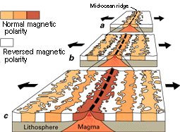 Figure 1: Alternating stripes of normally and reversely magnetized oceanic crust surrounding mid-ocean spreading ridges provide evidence of reversals in Earth's magnetic field over time.
![[reuse info]](/images/information_16.png)
A model is a simplified representation of a process or phenomenon that is used to further our understanding of that process or phenomenon. It may be physical in nature, such as the papier-mâché volcanoes many of us constructed in elementary school, or numerical, in which case lines of computer code studded with equations create a virtual representation of the subject under study.
Models are used widely in Earth and environmental science research because many of the questions of interest in these disciplines present spatial and temporal challenges that prevent us from addressing them directly. For example, we know from studies of magnetic minerals contained in oceanic crustal rocks (Fig. 1) that Earth's magnetic field reverses polarity from time to time, with the north pole becoming the south and vice versa. While the evidence for these flip-flops is clear, their cause is less so, and one of the difficulties of trying to figure out why the field reverses is that we cannot visit Earth's fluid outer core from which the magnetic field is thought to emanate. Not even the deepest borehole ever drilled, a >12.3 km deep oil well completed off the coast of Russia in 2011, comes anywhere close to reaching it. At a depth of 2890-5150 km, the outer core is permanently off-limits to humanity, observable only indirectly in features such as magnetic field lines that we can measure at Earth's surface and in the records of previous magnetic field orientations sealed in igneous rocks.
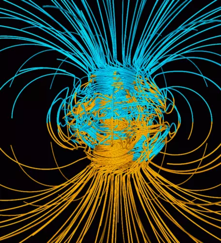 Figure 2: Numerical model simulation of Earth's magnetic field.
How then can we learn about the cause of magnetic polarity reversals? Geophysicists use numerical models to study this phenomenon. Simulating Earth's outer core as a churning sea of molten iron heated from below by a solid inner core, these models employ magnetohydrodynamic equations (equations governing the creation of magnetic fields by electrically conductive fluids) to generate magnetic field lines that vary in strength and orientation as the molten iron sloshes around in response to heating and Earth's rotation (Fig. 2; Glatzmaier, 2013). Comparison of the simulated field lines to Earth's actual magnetic field provides clues to the physical properties and behavior of the real system and brings us closer to a comprehensive understanding of how the magnetic field originates.
Another issue commonly encountered by Earth and environmental scientists is that many of the systems we seek to understand operate on spatial scales that may be regional or even global in extent. Take, for example, the San Andreas fault system that runs through the state of California. This fault and others closely related to it have been responsible for strong earthquakes that have killed scores of people and caused billions of dollars in property damages. It would be very helpful if we could somehow predict when and where future earthquakes will happen, but in order to do so, we need a better understanding of what causes faults to slip.
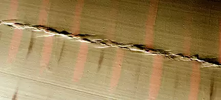 Figure 3: Physical model of strike-slip faulting created by shearing a layer of clay sitting atop two boards.
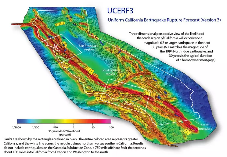 Figure 4: Map of earthquake probability in the state of California for the next 30 years. The San Andreas fault (red) shows the highest likelihood of a substantial rupture.
Just as spatial scales can present a variety of difficulties when studying aspects of the Earth system, the vast span of geologic time in relation to the length of a human life also causes challenges. Some processes occur so slowly that they are nearly impossible to detect. A good example is the gradual wearing away of entire mountain ranges by erosion, which typically occurs at rates measured in the microns per year (Fig. 5; see for example, Bierman and Caffee, 2001). Though modern global positioning satellite technology allows us to track horizontal and vertical surface motions that happen at rates of millimeters per year, no equipment has yet been invented that can sense changes occurring one thousand times more slowly. Only by looking at geologic evidence that has accumulated for thousands or perhaps even millions of years does landscape scale erosion make itself known. Numerical models that employ equations to describe a variety of erosional processes have been used to simulate landscape evolution, with the results compared to known topographic features in order to determine the rates at which these processes operate.
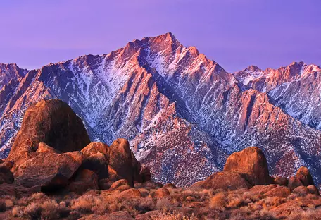 Figure 5: The Alabama Hills (foreground) and Sierra Nevada range (background) of eastern California have been sculpted by erosion over millions of years. Image by Steve Berardi.
![[creative commons]](/images/creativecommons_16.png)
A phenomenon that is difficult to study directly because it involves both a large spatial scale and a longtime scale is global climate change. In the last several decades there has been growing awareness that combustion of fossil fuels is contributing to a rapid warming of the globe. This warming is leading to the melting of glaciers and ice sheets, rising sea level, and changes in atmospheric circulation and associated weather patterns, and has the potential to cause major disruptions in water and food supplies, the extinction of species that cannot keep up with changing climates, and the poleward spread of diseases and parasites that historically have been confined to more tropical latitudes. Use of coal, oil, and natural gas is driving an uncontrolled experiment on our planet, the results of which we need to predict in order to plan for and possibly mitigate the most negative consequences, a majority of which will occur far into the future. Unfortunately, there do not exist multiple Earths orbiting the sun on which we can carry out various experiments to learn in advance what the results of different greenhouse gas levels will be. Nor do we have another planet that we can use as a control to see how climate might change in the absence of human activities. Our only remedy to this problem then is to use numerical models to simulate the impacts of increasing greenhouse gas levels (Fig. 6).
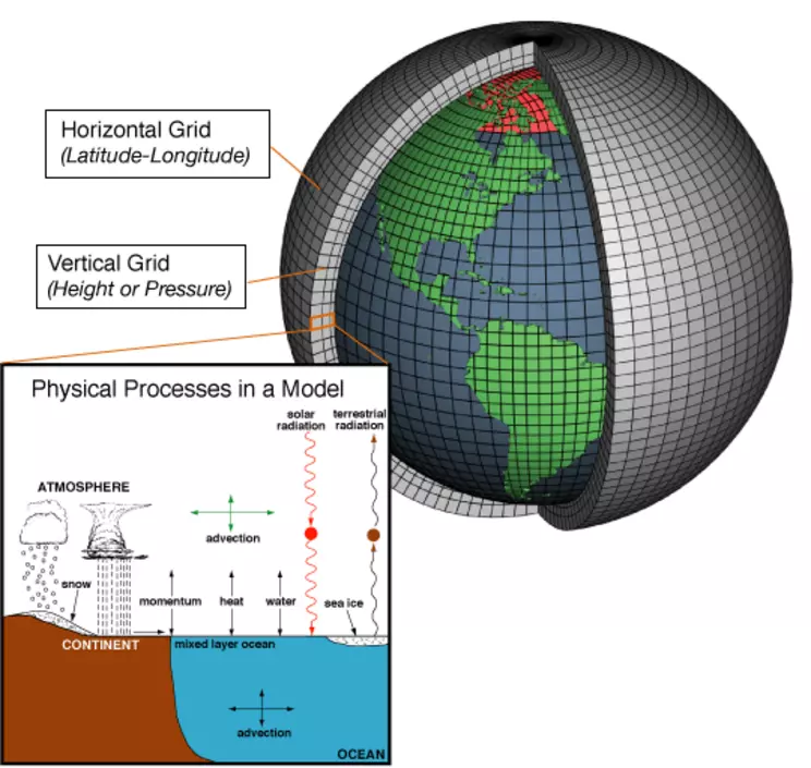 Figure 6: Numerical models of Earth's climate system allow scientists to explore how changing greenhouse gas levels in the atmosphere affect global temperature and precipitation patterns.
The advent of supercomputers in the 1980s initiated the climate modeling revolution, and continuing advances in computational power since that time have allowed ever better simulations of Earth system behavior. The most sophisticated models available today divide the oceans, atmosphere, and land surface into thousands of grid cells defined by latitude, longitude, and depth/elevation. These boxes contain water, air, or land and are allowed to exchange matter and energy with surrounding grid cells in response to changes in solar radiation and greenhouse gas levels. The models incorporate simplified topography as well as varying surficial materials such as forests, deserts, and ice sheets. To use them to predict future climate under different greenhouse gas level scenarios requires first that they demonstrate the ability to successfully simulate climate of the past, the evidence for which is contained in numerous biological and geological proxies such as tree rings and ice cores. Many of the models scientists have created have produced results sufficiently accurate to allow them now to be used to predict what climate will be like for a world in which carbon dioxide levels continue to increase. Though improvements remain to be made, the results of current model experiments are sobering and point to the importance of reducing humanity's carbon footprint in order to prevent catastrophically rapid climatic warming (Fig. 7).
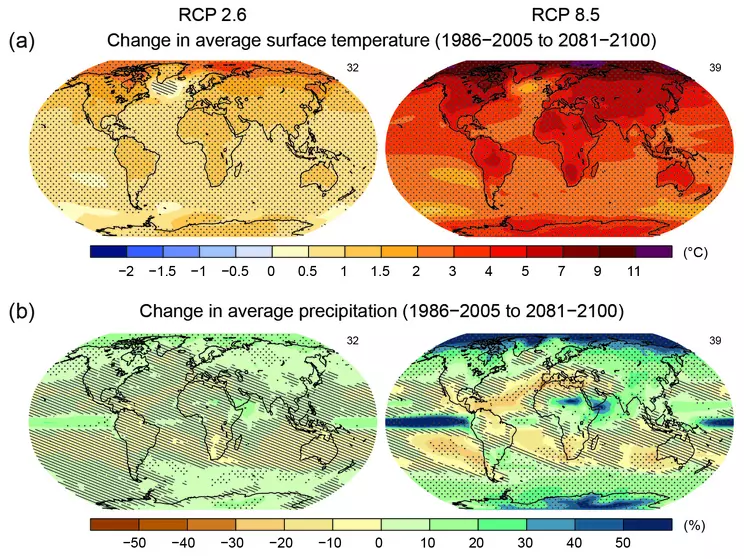 Figure 7: Results of numerical modeling experiments published in the 2014 Intergovernmental Panel on Climatic Change Assessment Report 5 indicate that increasing greenhouse gas levels will lead to a warmer planet with more variable precipitation values. RCP 2.6 is an experiment in which greenhouse gas levels peak between 2010 and 2020 and decline thereafter. RCP 8.5 represents a scenario in which greenhouse gas levels continue to rise throughout the 21st century.
To summarize, the purpose of numerical modeling in the Earth and environmental sciences is to allow us to:
- Simulate processes in locations inaccessible to humans.
- Simulate processes too large to allow the construction of physical models.
- Simulate processes too slow to permit human observation.
- Address critical environmental problems, such as anthropogenic climate change.
Focusing on Earth's climate system and on human activities that perturb it, this course will give you the tools to develop your own models of environmental processes and phenomena as well as to be able to evaluate the models of others whose work you may encounter as you embark on a scientific career. While we will not use the most sophisticated global climate models that require supercomputers to execute, there is still much to be learned from simple models of climate system components, and we will spend the next 10 weeks developing and experimenting with models on topics such as:
- Population growth and human use of resources
- What determines Earth's average surface temperature
- How life can regulate climate
- How ice sheets wax and wane in response to changes in solar radiation receipts at Earth's surface
- How changes in climate over time can be recorded in geologic proxies such as lake shorelines
- How measurements of borehole temperatures in Arctic permafrost contain information on recent global warming
- What the impacts of changing water temperature and salinity are on ocean circulation
- How carbon moves between different Earth reservoirs and what the impacts are of fossil fuel combustion
- Whether or not the "tragedy of the commons" is an inevitable byproduct of human resource use
Systems and their behavior
Climate is the long-term pattern of meteorological variables, such as temperature, rainfall, and wind speed, that characterizes a particular location on Earth's surface and is produced by complex interactions between the atmosphere, oceans, land surface (soils, rocks, and bodies of water), biosphere, and cryosphere (ice sheets and glaciers), along with solar energy. Earth's climate is an example of a complex system in that it is composed of multiple interacting components that together generate behaviors that are difficult to predict. Systems are made up of reservoirs that contain physical materials or quantities of energy as well as flows that transport those materials or that energy between the different reservoirs.
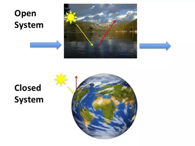 Figure 8: Open systems allow both matter and energy to flow across their boundaries whereas closed systems permit only energy to cross their boundaries. Here the blue arrows represent water, sediment, fish, and any other materials that enter and/or leave a lake. The yellow arrow represents incoming solar energy, and the red arrow represents both reflected solar energy as well as energy that was absorbed and then radiated back toward space.
Dynamic systems can exhibit a variety of different behaviors over time (Fig. 9) that are determined by differences in their inputs and outputs and by how these flows are related to the reservoirs to which they are attached. Steady state systems are characterized by inflows and outflows that are in complete balance such that no change occurs over time in the total amount of material contained within the reservoir. This does not mean that the material in the reservoir remains the same. Consider a lake fed by an inflow stream and drained by an outflow stream as an example. The water in the lake tomorrow will not be the same water as is in the lake today even though the lake remains the same size.
Systems in which the inflows are greater than the outflows and both have constant values exhibit linear growth. The opposite case, in which outflows are greater than inflows and both have fixed values yields linear decay. In some situations, inflows and outflows may depend on the sizes of the reservoirs to which they are attached. Population growth is a perfect example because the number of babies born in any given year depends on how many individuals of reproductive age already exist. The fewer reproducing pairs that exist, the fewer babies will be born, and the larger the population, the more babies will be born. Systems in which the inflows depend on the reservoir contents exhibit exponential growth, a type of increase that, unlike the constant rate of increase exhibited by linear growth, accelerates over time. Compounding interest is a financial example of the same phenomenon. Just as systems may exhibit exponential growth, they can also exhibit exponential decay. In this case, the outflows from the reservoir are dependent on the reservoir contents. A well-known geologic example of exponential decay is the radioactive decay of elements used in absolute dating of rocks and organic remains.
While the combination of inflows and outflows in some systems may cause reservoirs to grow or shrink over time, other systems exhibit oscillatory behavior in which the reservoir contents fluctuate between fixed values in a regularly repeating way. Earth's climate system includes several examples of oscillatory behavior, such as the cycle of daily heating and cooling caused by Earth's rotation through the rays of the sun as well as the cycle of the seasons. Now that we are aware of what systems are and of the different ways in which they may behave, we are ready to address how they might be simulated in a numerical model.
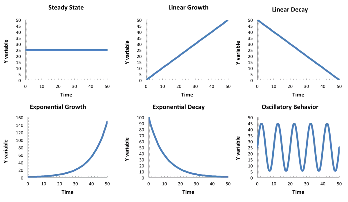 Figure 9: Dynamical systems can exhibit a variety of behaviors depending on the relative sizes of their inflows and outflows as well as whether those flows are dependent in any way on reservoir size.
Building numerical models
Creating a model requires a lot of careful thinking, research, and simple calculations. The starting point is always a question, such as "What would be the impact of doubling carbon dioxide levels in Earth's atmosphere on global average surface temperature?" or "How will water levels in an aquifer respond to varying rates of groundwater withdrawal?" In developing the central question that drives our inquiry, we begin to contemplate the sorts of information necessary to address it. Let us use the question about the aquifer as an example for how we go about the modeling process.
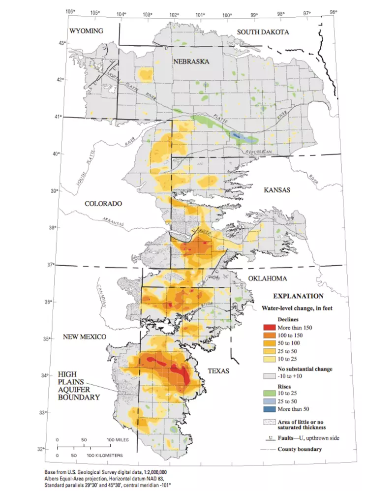 Figure 10: The High Plains Aquifer has been pumped extensively to irrigate wheat fields in the central United States.
To begin the modeling process, we create a sketch that represents our conceptual model of the aquifer system. Let us assume that the aquifer is unconfined and that it has an impermeable layer, called an "aquitard," at its base. Water is added through the infiltration of precipitation, accumulates in the aquifer, and leaves by discharge into a stream. The amount of water in the aquifer determines the height of the water table. Figure 11 depicts a cross-sectional sketch, but we will assume that the aquifer is really a three-dimensional entity.
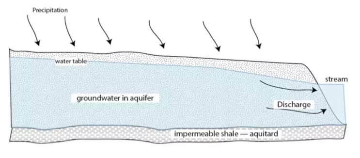 Figure 11: Conceptual model of an aquifer system.
Now that we have sketched our model, we need to figure out what the units are for the various parts of the system. It makes sense to represent the aquifer water in terms of volume - m3 or km3, depending on its scale. Given this, the flows in and out would have units of m3per unit of time or km3 per unit of time. We are interested in the long-term behavior of this aquifer, so it makes sense to use one year as the basic unit of time, giving the flows units of m3/yr or km3/yr. Note that in this step of defining the units, we are also defining the timescale of the system.
Next, we attempt to add some actual numbers to our model. For the precipitation inflow, we can get the volume of water per year that falls on the aquifer by knowing the average annual rainfall rate for the geographic location in which the aquifer resides and multiplying that value by the surface area over which the rain falls. Let us assume, for example, that the precipitation arrows in our conceptual model have a value of 0.3 m/yr, or 0.0003 km/yr, and that the surface area over which the rain falls is 500 km2 (recall that Figure 11 is a cross-section through what is actually a three-dimensional aquifer). This gives us a total of 500 km2 * 0.0003 km/yr = 0.15 km3/yr of rain falling onto the aquifer. We also need a starting volume of water in the aquifer, which we can get if we assume an average height of the water table above the aquitard (we'll use 100 m, or 0.1 km) and the porosity of the aquifer (porosity is the amount of pore space that can hold water between the bits of rock and/or sediment that constitute the aquifer; we will use 20% as our value). Combining these with the aerial extent of the aquifer to represent its full three-dimensional nature gives us 500 km2 * 0.1 km * 0.2 = 10 km3 contained within the aquifer.
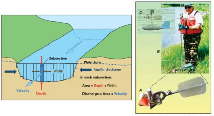 Figure 12: Stream base flow can be determined by using a current meter (right) to measure stream velocity and multiplying that value by the cross-sectional area of the stream (left).
` k = (D)/(V) `
Another approach to determining the percentage would be to make the assumption that the aquifer is in a steady state, neither increasing nor decreasing in volume, in which case the discharge would have to be equal to the amount of water added to the aquifer by precipitation - 0.15 km3/yr.
The percentage we would be looking for then would be:
` k = (D)/(V) = (0.15 (km^3)/(yr))/(10 km^3) = 0.015/(yr) `
Note that the units of k are yr-1, and for this reason, k is also known as a rate constant.
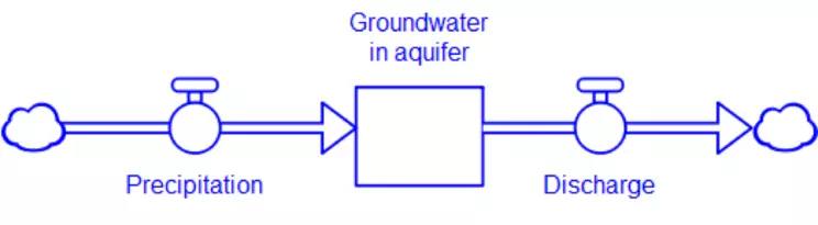 Figure 13: STELLA representation of a simple aquifer model.
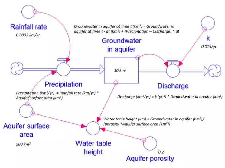 Figure 14: Modified STELLA model that incorporates the dependency of the discharge flow on the rate constant and the amount of groundwater contained within the aquifer.
To make the model more complete, we can add a few items to allow the calculation of the precipitation flow from the aquifer surface area and rainfall rate and the determination of the water table height from the volume of groundwater in the aquifer, the aquifer surface area, and the porosity (Fig. 14). Recognizing that we earlier determined that ` k = (D)/(V) `, we have rearranged this equation to allow the model to calculate the discharge from the rate constant multiplied by the volume of groundwater in the aquifer: ` D = kV `. Note that the additional elements we have added to the model are represented in STELLA by circles. These are known as converters and are used to hold values of constants or equations. We have also drawn a number of pink arrows on the model. These are known as action connectors and show the dependencies between different variables. For example, there are two action connectors linked to the Discharge flow arrow, one from the Groundwater in aquifer reservoir and one from the converter circle holding the value of the rate constant k. These action connectors allow the STELLA software to recognize that the Discharge flow arrow depends on these two items.
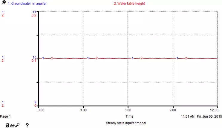 Figure 15: Results of the STELLA run show that the aquifer system is in steady state, neither gaining nor losing volume over time.
To test the model, we can run it and graph the aquifer reservoir and the water table height, both of which should stay constant over time since we designed this model with the assumption that the aquifer system is in a steady state. As Figure 15 shows, this is indeed the case, and the groundwater in aquifer volume remains 10 km3 throughout the model run while the water table height holds steady at 0.1 km. Having convinced ourselves that the model is working correctly, we can now go on to explore the impact of pumping on the aquifer volume. To do this, we incorporate a second outflow from the groundwater in aquifer reservoir that will remove water from the system for a limited period of time (Fig. 16).
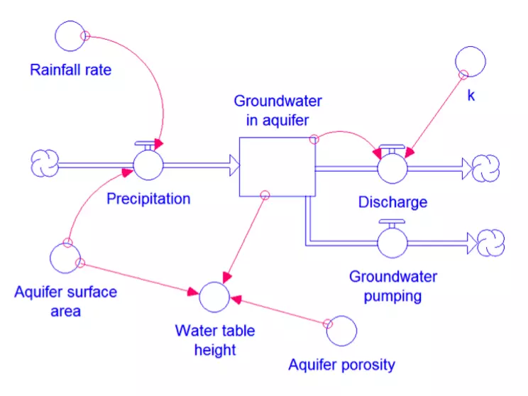 Figure 16: STELLA model modified to include groundwater pumping for a 35-year period near the beginning of the simulation.
We have to assign some numbers to this pumping flow. We are going to assume that it will not exceed the steady state precipitation rate, but this limit is really just an arbitrary decision. If we were truly trying to model the depletion of the High Plains Aquifer, we would need to acquire water usage data from farmers. We are going to stick to a very simple model here and set the pumping rate at 0.09 km3/yr from years 10 through 45 of the model run. The pumping flow will not depend on any other parameter in the model - it will simply represent the demand for groundwater. Figure 17 shows how this 35-year interval of pumping affects the steady state aquifer condition we previously modeled.
As we can see, as soon as the groundwater pumping begins, the water table declines and so does the discharge (because it depends on the amount of water in the aquifer). Once the groundwater pumping ends, the system restores to the steady state condition. The restoration is rapid at first, and then slows as it gets closer to the steady state values. This speed of recovery is a measure of the response time of this system, or the time it takes for a system to accomplish about 2/3 of its return to steady state (Because the system returns to steady state asymptotically, it is difficult to determine when it has actually arrived at the steady state value. For this reason, scientists have settled on a value of about 2/3 of the total response in order to be able to compare different systems to one another). We can determine this value by taking the reciprocal of the rate constant: 1/k - 66.67 years in this case. Now that we have created this simple model of an aquifer system, there are many possibilities for refining it, such as making the rainfall and groundwater pumping change with the seasons and incorporating more realistic values for the recharge, discharge, and aquifer size.
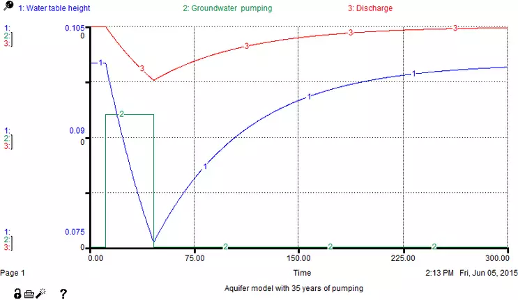 Figure 17: Groundwater pumping (green line) results in a decline in the water table and in stream discharge. Shutting off the pumping allows the system to slowly recover to its pre-disturbance state.
Summary
Let us summarize the steps involved in creating our simple groundwater model, which together amount to a sort of recipe for model building in general.
- We always start with a question that involves some kind of system changing over time.
- We make a sketch of what the system involves - a conceptual model - and make it as simple as possible.
- We figure out what quantity will be monitored in the system, meaning we define the units to be used. We also consider what timescale seems most appropriate for the system we are modeling.
- We add numbers and equations to the different system components, making sure that all the units work out. In doing this, it is often useful to design the model to be in a steady state to begin with as this makes experimentation easy.
- We translate the conceptual model into the system components used in STELLA - reservoirs, flows, converters, and action connectors.
- Once we have built our STELLA model and incorporated all of the necessary values of constants and equations linking the different variables, we go on to test the model and see if the results make sense. If the model is supposed to reflect steady state, then there should be no change in the values of any of the variables.
- If the results are as expected, we can then go on to experiment with the model and incorporate additional complexity, exploring the response of the system to each change we make.
Why do we use a computer to model?
Our first modeling example was extremely simple - a bathtub model of an aquifer - and you might be asking yourself whether it would not have been easier to just use a little algebra to figure out the amount of water in the aquifer at some point in the future, rather than to go to the trouble of constructing a STELLA model. The answer to this question is that even with this extremely simple system, the math becomes challenging fairly quickly when we are interested in how that system might evolve over time in response to changing inputs or outputs. To see that this is so, let us take a look at the math involved in studying this problem. We will use the letter V to denote the volume of water in the aquifer, t to denote time, i to represent the inflowing precipitation, and o to represent the outgoing discharge to the stream.
The change in volume in the aquifer with time (` (dV)/(dt) `) is equivalent to the inflow minus the outflow:
` (dV)/(dt) = i - o `
Recall, however, that the outflow really depends on how much water is in the aquifer, and that we can use a constant of proportionality, also known as the rate constant (k), to determine its value:
` o = kV `
If we now substitute the equation for the outputs into the initial equation, we get:
` (dV)/(dt) = i - kV `
This is a first-order homogeneous differential equation that can be solved using a little calculus. The first step is to integrate both sides:
`int (dV)/(dt) = int i - kV`
To do this, we need to separate the variables so that all terms having to do with volume are on the left-hand side and all terms having to do with time are on the right-hand side:
`int (dV)/(i - kV) = int dt `
Carrying out this integration yields the following equation, where C is the constant of integration and e is a constant that is the base of the natural logarithm function and has a value of 2.718:
` V(t) = (i)/(k) + Ce^(-kt) `
We can evaluate the constant of integration by looking at its value when time equals 0 years. Substituting 0 in for t in the equation above yields:
` V(0) = V_0 = (i)/(k) + C `
Thus ` C = V_0 - (i)/(k) `
The final equation that describes the evolution of the aquifer volume over time can then be determined by substituting the value of the constant of integration into the previous equation to yield:
` V(t) = (i)/(k) + (V_0 - (i)/(k))e^(-kt) `
This equation is known as the analytical solution. As long as we know the values of the inflow, the rate constant, and the initial value of the aquifer volume, we can determine the value of the equation for any time t and know what the volume of water in the aquifer is at that time.
As you can see from this example, the mathematics for even this simple model are relatively involved and require calculus to arrive at the solution. Now suppose that the system we are interested in modeling consists of multiple reservoirs interconnected in a variety of different ways, and that the inflows and outflows change over time. You can probably imagine how challenging it would be to develop the analytical solution equations necessary to keep track of the volumes of the different reservoirs over time. The beauty of numerical modeling and of the STELLA software in particular is that we do not have to; we can allow the computer to do the heavy lifting for us, and we will never have to use anything more complicated than simple algebra.
Limitations of models
Numerical models are wonderful tools for analyzing complex systems that operate over a variety of spatial and temporal scales. However, it is also important to remember that they are only as good as the assumptions that go into building them. Many an inexperienced modeler has developed an apparently elegant and sophisticated code in which a misplaced parenthesis in an equation or a failure to ensure a consistency of units throughout the model has yielded an unusual result. Rather than immediately recognizing that the model behavior is spurious due to an error of this sort, the inexperienced person is likely to attempt to explain it, sometimes invoking parameters that are not even included in the model. Because this is such a common occurrence, we find it useful to remind students of a few rules of thumb borrowed here from Cross and Moscardini (1985):
- Remember, all models are partial, they never represent the entire system.
- Models are usually initially built for a specific purpose; be careful, therefore, of using them for purposes other than originally intended.
- DO NOT FALL IN LOVE WITH YOUR MODEL!!!
- Take your model results with a grain of salt unless directly validated in some way. (This is often difficult to do in Earth and environmental science, because we may not be able to validate to the extent we would like to because processes occur on too large of a spatial scale or too long of a temporal scale).
- Do not distort reality to fit the model.
- Do not retain discredited models.
- Do not extrapolate beyond the region of validity of your model hypotheses.
- Keep ever-present the distinction between models and reality.
- Be flexible and willing to modify your model as the need arises.
- Keep your objectives ever present by continually asking yourself, "What am I trying to do?"
If you can remind yourself to always start with the simplest possible model that will address the question you are seeking to answer, to add complexity gradually, and to critically evaluate your results at every step, you will avoid much difficulty and perhaps even heartbreak as you work toward a better understanding of the world around you. Numerical modeling is as much an art as it is a science. It requires mathematical skill, experience, and intuition. Because intuition is only gained with experience, modeling can be quite frustrating at first. We wish to reassure you that any exasperation you feel is both normal and expected. As you continue through this course, you will grow in experience and will become more confident in your abilities to both identify and solve problems. Let us get to work!
References
Bierman, P.R., and Caffee, M., 2001, "Slow rates of rock surface erosion and sediment production across the Namib Desert and escarpment, southern Africa," American Journal of Science, v. 301, p. 326-358.
Cross, M., and Moscardini, A.O., 1985, Learning the Art of Mathematical Modeling, New York: Halstead Press, 155 p.
Ghosh, A., and Holt, W.E., 2012, "Plate Motions and Stresses from Global Dynamic Models," Science, v. 335, p. 838-843.
Glatzmaier, G.A., 2013, Introduction to Modeling Convection in Planets and Stars: Magnetic Field, Density Stratification, Rotation, Princeton University Press, 328 p.
Jolivet, R., Simons, M., Agram, P.S., Duputel, Z., and Shen, Z.-K., 2015, "Aseismic slip and seismogenic coupling along the San Andreas Fault," Geophysical Research Letters, v. 42, p. 297-306.


