For the Instructor
These student materials complement the Modeling Earth Systems Instructor Materials. If you would like your students to have access to the student materials, we suggest you either point them at the Student Version which omits the framing pages with information designed for faculty (and this box). Or you can download these pages in several formats that you can include in your course website or local Learning Managment System. Learn more about using, modifying, and sharing InTeGrate teaching materials.Unit 4 Reading: Daisyworld
by Louisa Bradtmiller, Macalester College, and Kirsten Menking, Vassar College
This week's project uses a model of a simple planet where only two organisms grow: black daisies and white daisies. Since the daisies have different albedos, they affect local radiative balance and therefore local (and average planetary) temperature differently. The lab explores concepts of feedbacks, homeostasis, thresholds, and the possibility that a single system may have multiple stable states, and it draws on concepts encountered in the population and climate modeling labs of the last two weeks.
The faint young sun paradox
 Figure 1: Nuclear fusion in the sun converts hydrogen atoms into helium, releasing electromagnetic radiation that travels throughout the solar system and warms Earth.
 ![[creative commons]](/images/creativecommons_16.png)
The Gaia Hypothesis
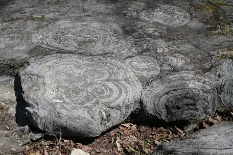 Figure 2: Fossils of photosynthetic bacteria, called stromatolites, demonstrate that early Earth had liquid water. (Photo by Michael C. Rygel via Wikimedia Commons.)
Daisyworld
Early iterations of the Gaia hypothesis attracted interest, but also criticism from those who did not believe that simple organisms could act with such an organized "purpose." In 1983, Lovelock teamed up with Andrew Watson to show that organisms need not "know" what they are doing, but still might modify the environment in a stabilizing way. To illustrate their point, Watson and Lovelock created a simple model of a fictional planet with two species—black and white daisies—whose albedos and temperature-sensitive growth rates modify planetary temperature (Fig. 3).
 Figure 3: Daisyworld, as envisioned by scientists at NASA's Goddard Space Flight Center. White daisies have a much higher albedo than black daisies, causing them to reflect more incoming solar energy.
The growth of daisies is governed by the expressions:
` (da_w)/dt = a_w(x beta_w - gamma) ` (Eqn. 1)
` (da_b)/dt = a_b(x beta_b - gamma) `
where aw and ab are the areas of ground covered by white and black daisies, x is the proportion of bare ground still available for colonization, ` beta ` is a growth function dependent on temperature, and ` gamma ` is a death rate. You may recognize these equations as being quite similar to those we used to model populations in week 2 of the class.
In equation 1 above, x can be determined from:
` x = p - a_b - a_w ` (Eqn. 2)
where p is set equal to 1. X and the areas of ground covered by the daisies are therefore fractional values lower than 1. The growth function ` beta ` is specified by:
` beta_y = 1 - 0.003265(22.5 - T_y)^2 ` (Eqn. 3)
where Ty is the temperature of the black or white daisies. Since the white and black daisies have different albedos, they have different temperatures, and for this reason, each color must have its own ` beta_y ` growth function.
Because of its parabolic shape, the growth function acts as both a positive and a negative feedback. Initially, as the planet warms due to the increasing luminosity of the sun, a small population of black daisies warms sufficiently to begin growing. As these daisies grow, their presence further warms the planet due to their low albedo, leading to still more growth in a positive feedback loop. Due to the parabolic shape of the growth function, however, continued growth of black daisies slows as temperatures become too warm for them. Eventually, temperatures are warm enough to allow the white daisies to begin to grow despite their high albedos. Their growth acts as a negative feedback. The more these daisies grow, the more they act to cool the warming planet.
The energy balance of Daisyworld can be determined by equating the amount of energy coming in from the sun with the amount of energy going out via radiation:
` SL(1-A) = sigma (T_d + 273)^4 ` (Eqn. 4)
where S is the solar constant (917 W/m2), L is a function that ramps up the solar output over time, A is the planetary albedo, ` sigma ` is the Stefan-Boltzmann constant (5.67e-8 W/m2K4), and Td is the temperature of Daisyworld. This is simply a rearranging of one of our basic energy balance equations from last week.
The planetary albedo is derived by taking the weighted average of the albedos of the black and white daisies and of bare ground (Aw, Ab, and Ag are albedos; aw, ab, and x are fractional areas covered by daisies or bare ground):
` A = A_w*a_w + A_b*a_b + A_g*x ` (Eqn. 5)
Watson and Lovelock determine the local temperature (Ty) of bare ground, white or black daisies from the expression:
` (T_y + 273)^4 = q(A - A_y) + (T_d + 273)^4 ` (Eqn. 6)
where q is a positive constant described below. To show that using this equation for local temperature is valid in terms of the overall energy balance for the planet, they perform the following calculations:
The total energy radiated by Daisyworld to outerspace (F) is equivalent to the sum of the energies radiated from each type of ground cover (i.e., bare ground, black daisies, or white daisies):
` F = sum_(y) a_ysigma(T_y + 273)^4 ` (Eqn. 7)
substituting equation 6 above into equation 7 gives:
` F = sum_(y) a_ysigma[q(A - A_y) + (T_d + 273)^4] `
so
` F = sum_(y) a_ysigmaqA - sum_(y) a_ysigmaqA_y - sum_(y) a_ysigma(T_d + 273)^4 `
In this equation, `sigma`, q, A, and Td are all constants that can be pulled out of the summations to give:
` F = sigmaqAsum_(y) a_y - sigmaqsum_(y) a_yA_y - sigma(T_d + 273)^4sum_(y) a_y `
but
` sum_(y) a_y = 1 `
because the sum of all of the areas on the planet is 1, and
` sum_(y) a_yA_y = A `
because the planetary albedo, A, is equal to the area-weighted average albedo of the black and white daisies and of bare ground, so
` F = sigmaqA - sigmaqA - sigma(T_d + 273)^4 `
or
` F = sigma(T_d + 273)^4 `
Since the final value for F is equivalent to SL*(1-A), the planet can be seen to be in radiative balance using equation 6 for local temperature.
To understand the meaning of the q constant, Watson and Lovelock eliminate the planetary albedo term between equations 4 and 6:
` sigma(T_d + 273)^4 = SL(1 - A) ` (Eqn. 4)
so
` A = 1 - (sigma(T_d + 273)^4)/(SL) `
but
` (T_y + 273)^4 = q(A - A_y) + (T_d + 273)^4 ` (Eqn. 6)
so
` A = ((T_y + 273)^4 - (T_d + 273)^4)/q + A_y `
so, setting these 2 equations equal,
` 1-(sigma(T_d + 273)^4)/(SL) = ((T_y + 273)^4 - (T_d + 273)^4)/q + A_y `
Multiplying both sides by q gives:
` q[1 - (sigma(T_d + 273)^4)/(SL)] = (T_y + 273)^4 - (T_d + 273)^4 + A_yq `
` q[1 - (sigma(T_d + 273)^4)/(SL)] - A_yq + (T_d + 273)^4 = (T_y + 273)^4 `
` (T_y + 273)^4 = q(1 - A_y) + (T_d + 273)^4*(1 - (qsigma)/(SL)) ` (Eqn. 8)
In the case where q = 0, the planet is a perfect conductor of absorbed radiation. In other words, excess energy absorbed in areas covered by black daisies is conducted away to areas covered by white daisies to create a planet with a perfectly uniform distribution of surface energy.
Plugging q = 0 into equation 8 above gives
` (T_y + 273)^4 = (T_d + 273)^4 `
In other words, the local temperature (Ty) is everywhere equivalent to the average planetary temperature (Td).
If on the other hand ` q = (SL)/sigma `, then there is no heat transfer between the different daisy species or the ground. Plugging this into equation 8 gives:
` (T_y + 273)^4 = (SL)/sigma (1 - A_y) + (T_d + 273)^4 * (1 - (SLsigma)/(sigmaSL)) `
the latter half of this equation goes to 0, to give:
` (T_y + 273)^4 = (SL)/sigma (1 - A_y) `
So in this situation, the local temperatures are determined by the local radiation balance.
Watson and Lovelock use a value intermediate between 0 and ` (SL)/sigma ` for q to allow for some conduction from black daisy areas to white daisy areas. That value is ` 0.2(SL)/sigma `.
References
Kump, L. R., J. F. Kasting and R. G. Crane, 2010, The Earth System, 3rd Edition. San Francisco: Prentice Hall.
Lovelock, J.E., 1972, "Gaia as seen through the atmosphere." Atmospheric Environment (Elsevier) v. 6, p. 579–580.
Lovelock, J.E.; Margulis, L., 1974, "Atmospheric homeostasis by and for the biosphere: the Gaia hypothesis." Tellus. Series A, Stockholm: International Meteorological Institute, v. 26, p. 2–10.
Sagan, C.; Mullen, G., 1972, Earth and Mars: Evolution of Atmospheres and Surface Temperatures." Science, v. 177, p. 52–56.
Watson, A.J., and Lovelock, J.E., 1983, "Biological homeostasis of the global environment: the parable of Daisyworld," Tellus, v. 35B, p. 284–289.


