Tensors: Stress, Strain and Elasticity

by Pamela Burnley, University of Nevada Las Vegas

Outline

Introduction

The Stress Tensor
The Strain Tensor
Elasticity
Literature

Introduction

Many physical properties of crystalline materials are direction dependent because the arrangement of the atoms in the crystal lattice are different in different directions. If one heats a block of glass it will expand by the same amount in each direction, but the expansion of a crystal will differ depending on whether one is measuring parallel to the a-axis or the b-axis. For this reason properties such as the elasticity and thermal expansivity cannot be expressed as scalars. We use tensors as a tool to deal with more this complex situation and because single crystal properties are important for understanding the bulk behavior of rocks (and Earth), we wind up dealing with tensors fairly often in mineral physics.

What is a Tensor

A tensor is a multi-dimensional array of numerical values that can be used to describe the physical state or properties of a material. A simple example of a geophysically relevant tensor is stress. Stress, like pressure is defined as force per unit area. Pressure is isotropic, but if a material has finite strength, it can support different forces applied in different directions. Figure 1 below, illustrates a unit cube of material with forces acting on it in three dimensions. By dividing by the surface area over which the forces are acting, the stresses on the cube can be obtained. Any arbitrary stress state can be decomposed into 9 components (labeled σ_ij). These components form a second rank tensor; the stress tensor (Figure 1).

Tensor math allows us to solve problems that involve tensors. For example, let's say you measure the forces imposed on a single crystal in a deformation apparatus. It is easy to calculate the values in the stress tensor in the coordinate system tied to the apparatus. However you may be really interested in understanding the stresses acting on various crystallographic planes, which are best viewed in terms of the crystallographic coordinates. Tensor math allows you to calculate the stresses acting on the crystallographic planes by transforming the stress tensor from one coordinate system to another. Another familiar tensor property is electrical permittivity which gives rise to birefringence in polarized light microscopy. You are probably familiar with the optical indicatrix which is an ellipsoid constructed on the three principle refractive indices. The refractive index in any given direction through the crystal is governed by the dielectric constant K_ij which is a tensor. The dielectric constants "maps" the electric field E_j into the electric displacement D_i :

Were k₀ is the permitivity of a vacuum. D_i can be calculated from E_j as follows:

 

D₁ = k_oK₁₁E₁ + k_oK₁₂E₂ + k_oK₁₃E₃

D₂ = k_oK₂₁E₁ + k_oK₂₂E₂ + k_oK₂₃E₃

D₃ = k_oK₃₁E₁ + k_oK₃₂E₂ + k_oK₃₃E₃

 

So you can see that even if E₁ is the only non-zero value in the electric field, all the components of D_i may be non-zero.

Rank of a Tensor

Tensors are referred to by their "rank" which is a description of the tensor's dimension. A zero rank tensor is a scalar, a first rank tensor is a vector; a one-dimensional array of numbers. A second rank tensor looks like a typical square matrix. Stress, strain, thermal conductivity, magnetic susceptibility and electrical permittivity are all second rank tensors. A third rank tensor would look like a three-dimensional matrix; a cube of numbers. Piezoelectricity is described by a third rank tensor. A fourth rank tensor is a four-dimensional array of numbers. The elasticity of single crystals is described by a fourth rank tensor.

Tensor transformation

As mentioned above, it is often desirable to know the value of a tensor property in a new coordinate system, so the tensor needs to be "transformed" from the original coordinate system to the new one. As an example we will consider the transformation of a first rank tensor; which is a vector. If we have a vector P with components p₁, p₂, p₃ along the coordinate axes X₁, X₂, X₃ and we want to write P in terms of p′_1, p′_2, p′₃ along new coordinate axes Z₁, Z₂, Z₃, we first need to describe how the coordinate systems are related to each other. This can be done by noting the angle between each axis of the new coordinate system and each axis of the old coordinate system; altogether there will be 9 angles, three of which are illustrated in 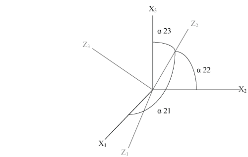Figure 2:

 

 

 

 

We can then express p′_1, p′_2,and p′₃ in terms of p₁, p₂, and p₃:

 

 

 

p′₁ = p₁cos α₁₁ + p₂cos α ₁₂ + p₃cos α ₁₃
 

p′₂ = p₁cos α ₂₁ + p₂cos α ₂₂ + p₃cos α ₂₃

p′₃ = p₁cos α ₃₁ + p₂cos α ₃₂ + p₃cos α ₃₃ 
 

 

 

 

 

To abbreviate, we replace the cosα with "a" (e.g cosα₂₁ = a₂₁) and notice that each equation can be rewritten as:

 

 

 

 

which can be further condensed to:

 

 

If we utilize Einstein's summation convention, we can leave out the summation symbol and get:

 

(1) p′_i = a_ijp_j (i,j = 1, 2, 3) .

 

There is a similar process for transforming a second rank tensor, but calculating a formula for the transformation by the same means that we transformed the vector above would be quite laborious. There is a more convenient shortcut. Just as the dielectric constants "maps" the electric field Ej into the electric displacement Di, we can imagine a second rank tensor T_kl that takes Q_l and produces P_k in a given coordinate system:

(2) P_k =T_klQ_l

 

We want to find the values for this second rank tensor in a new coordinate system. In the new coordinate system this tensor, T′_ij will produce P′_i from Q′_j, where P′_i and Q′_j are the transformed versions of P_k and Q_l.

(3) P′_i=T′_ijQ′_j

 

We already know how to transform P_i into P_k:

(4) P′_i = a_ikP_k

 

 

and since

(5) P_k = T_klQ_l 
 

(6) P′_i = a_ik T_klQ_l

 

To transform Q′_jto Q_l we need only to realize that the direction cosines to go from the new coordinate system back to the old coordinate system are the same as those used to go from old to new, except the indices will be reversed. So:

(7) Q_l= a_jlQ′_j

 

which we can then substitute into the equation above and get

(8) P′_i = a_ikT_kla_jlQ′_j 
 

 

The tensor we are looking for is T′_ij:

(9) P′_i = T′_ijQ′_j 
 

 

Substituting (9) into the left hand side of (8) and dividing by Q_j we get

(10) T′_ij = a_ika_jlT_kl 
 

 

The Identity Tensor

A valuable tool in tensor math is the identity tensor, which is referred to as the Kronecker delta:

 

 

 

It is abbreviated as:

 

 

 

The Stress Tensor

Stress is defined as force per unit area. If we take a cube of material and subject it to an arbitrary load we can measure the stress on it in various directions (figure 4). These measurements will form a second rank tensor; the stress tensor.

 

 

 

 

 

 

 

The Eigen values of σ_ij ; represented as σ₁ , σ₂ , σ₃ are referred to as the principle stresses.

 

 

 

 

 

 

 

The Eigen vectors are the principle stress directions known as the maximum, intermediate and minimum principle stresses respectively; in geology compression is considered positive and the maximum compressive stress is referred to as σ₁. However, in engineering and physics, tension is considered positive so the maximum compressive stress is referred to as σ_3. Therefore, it is important to be aware of which sign convention is being used. A cube with its edges parallel to the principle stress directions experiences no sheer stresses across its faces.

An important property of the stress tensor is that it is symmetric:

σ_ij = σ_ji

Intuitively, this can be seen if one images shrinking the cube in Figure 4 to a point. If the cube is infinitesimally small, the forces across each face will be uniform. If the cube is to remain stationary the normal forces on opposite faces must be equal in magnitude and opposite in direction and the shear tractions which would tend to rotate it must balance each other. So for example, if σ₁₃ is not equal in magnitude to σ_31,the cube will spin around the X₂ direction. Therefore, it is only necessary to find 6 of the components of the tensor.

Important concepts are often used are deviatoric stress and hydrostatic pressure. Any stress tensor may be broken into two parts

 

 

 

 

 

 

 

where 

p = ( σ₁₁ + σ₂₂ + σ₃₃ ) / 3)

Using the Kronecker delta notation this may be written as

σ_ij = σ_ij(dev) + pδ_ij .

The Strain Tensor 
 

 

Strain is defined as the relative change in the position of points within a body that has undergone deformation. The classic example in two dimensions is of the square which has been deformed to a parallelepiped.

Let us examine the movement of a point on the corner of the square (m) which moves to (m'): 

In order for this analysis to work we must only consider infinitesimally small strains. We will call the original length of the side of the square X₁. We will call the component of the displacement (d) of m to m' resolved onto the X₁ axis Δd₁and the amount of the the component of d resolved onto the X₂ axis Δd_2.A simple way to measure the strain would be to compare Δd₁ with X₁ and Δd₂ with X₁, etc.

We can represent this quantity by e₁₁

 

or more generally:

 

 

 

 

 

Since ∆d₂ is very small , 

 

(∆d₂/∆X₁) ≈ (∆d₂/(∆X₁ + ∆d₁)) = tanϴ.

For very small angles tanϴ = ϴ and therefore e₂₁ = ϴ. Now imagine that instead of being deformed, the initial square had been simply rotated around the origin, the values e_ij i≠j would still be non-zero. For this reason, strain is characterized by a tensor ϵ _ij from which the rigid body rotation has been subtracted. Therefore we can write:

ϵ _ij = e_ij - ῶ_ij

where ῶ_ij is the rigid body rotation andϵ _ij is defined as the strain.

ϵ _ij = ½(e_ij + e_ji)

ῶ_ij = ½(e_ij – e_ji)

For the two-dimensional case:

 

 

 

ϵ _ij is a symmetric tensor and ῶ_ij is an antisymmetric tensor; the leading diagonal ofῶ_ij is always zero.

The tensor ϵ _ij has Eigen values which are called the principal strains (ϵ₁, ϵ₂, ϵ₃). The Eigen vectors lie in the three directions that begin and end the deformation in a mutually orthogonal arrangement. If the Eigen vectors are initially of length 1 then in the end they are length:

1 + ϵ_i.

Strain lends itself well to geometric representation. Think of a unit sphere which has been deformed. By inspection, one could find the three orthogonal directions that have remained orthogonal in the deformation. The length of radial lines parallel to those orthogonal directions (X₁, X₂, X₃) will have changed length such that:

X₁^' = X₁(1 + ϵ₁)

X₂^' = X₂(1 + ϵ₂)

X₃^' = X₃(1 + ϵ₃).

If we substitute the new dimensions into the equation for the sphere in this particular reference frame:

X₁² + X₂² + X₃² = 1 .

 

 

We get

(X₁^{' 2})/(1 + ϵ₁)² + (X₂^{' 2})/(1 + ϵ₂)² + (X₃^{' 2})/(1 + ϵ₃)² = 1

This is the equation of an ellipsoid, which is called the strain ellipsoid. Often geologists will use statistical studies of the shapes of pebbles, certain types of sand particles, and other natural objects which were probably originally round, to determine the strain which a particular body of rock has undergone.

 

Elasticity

 

Unlike stress and strain, elasticity is an intrinsic property of a material. The elastic properties of Earth materials affects everything from the variation of density with depth in the planet to the speed at which seismic waves pass through the interior. Ultimately the elastic properties of a material are governed by the arrangement and strength of the bonds between the atoms that make up the material. Elasticity is the property of "reversible deformation". If the deformation in a body under stress does not exceed a certain limit, called the elastic limit, the body will return to its initial shape when the stress is removed. If the amount of stress (σ) is infinitesimaly small then the amount of strain (ϵ), which is also infinitesimal, is linearly proportional to the strain and may be written as:

ϵ = sσ

or

σ = cϵ

Where s is the elastic compliance and c is the elastic stiffness. In order to relate two second rank tensors, a fourth rank tensor is necessary.

ϵ_ij = s_ijkl σ_kl

or

σ_ij = c_ijkl­ ϵ_kl

To calculate ϵ_ij for the three-dimensional case we would begin like so:

ϵ₁₁ = S₁₁₁₁σ₁₁ + S₁₁₁₂σ₁₂ + S₁₁₁₃σ₁₃ + S₁₁₂₁σ₂₁ + S₁₁₂₂σ₂₂ + S₁₁₂₃σ₂₃ +

S₁₁₃₁σ₃₁ + S₁₁₃₂σ₃₂ + S₁₁₃₃σ₃₃

Notice that even if all σ_ij = 0 except σ_11, that most ϵ_ij ≠ 0 . This can be seen if you take a square and pull on it from only one direction;

 

 

 

 

it strains in all directions.
For the three-dimensional case there are 81 terms in a fourth rank tensor. However, both stress and strain are symmetric tensors; σ_ij = σ_ji and ϵ_ij = ϵ_ji each only has 6 independent terms. There are only 6 equations needed to calculate ϵ_ij from σ_ij and in each equation there will only be 6 independent terms. Therefore, there can be no more than 36 independent values in S_ijkl. For convenience, a matrix notation is used. The subscript is broken into two parts:

S_ij._kl

and abbreviated as follows:

 

To avoid the appearance of factors in the equations, the following factors are introduced into the matrix notation:

S_ijkl­ = S_mn for m, n = 1, 2, or 3

2S_ijkl­ = S_mn for m or n = 4, 5, or 6

4S_ijkl­ = S_mn for m and n = 4, 5, 6

2ϵ_ij = ϵ_m for m = 4, 5, or 6

 

 

 

In matrix notation the equation for obtaining strain from stress is:

ϵ_i = S_ijσ_j ( i,j = 1, 2, . . . 6)

and stress from strain is:

σ_i = C_ijϵ_j ( i,j = 1, 2, . . . 6)

 

 

The compliances and stiffnesses are written as an array; for example for S_ij

 

As I mentioned above, ϵ_ij and σ_ij are symmetric and therefore the number of independent coefficients is reduced from 81 to 36. Because of "compatibility relations," which say that material will deform continuously, the number is reduced to 21. If the material being deformed is symmetric the number of coefficients is even further reduced. For an isotropic material, one that behaves the same in any orientation, there are only two quantities necessary. These are Young's Modulus E, and G the Shear Modulus; all the coefficients may be expressed in terms of them.

S₁₁ = 1/E

2(S₁₁ - S₁₂) = 1/G

 

Or alternatively,

S₁₂ = ν/E

where ν is Poisson's Ratio

ν = (E/2G) – 1.

Therefore, for an isotropic material:

ϵ₁ = (1/E)(σ₁ – ν(σ₂ + σ₃))

ϵ₂ = (1/ E)(σ₂ – ν(σ₁ + σ₃))

ϵ₃ = (1/ E)(σ₃ – ν(σ₂ + σ₁))

ϵ₄ = (1/G)σ₄

ϵ₅ = (1/ G)σ₅

ϵ₆ = (1/ G)σ₆

 

From these equations it becomes obvious that for isotropic materials the directions of the principal stresses are the same as those for the principal strains. If a polycrystalline rock is large compared to the size of its constituent grains and does not have a preferred crystallographic orientation it will in general behave as an isotropic solid.

Elastic Constants

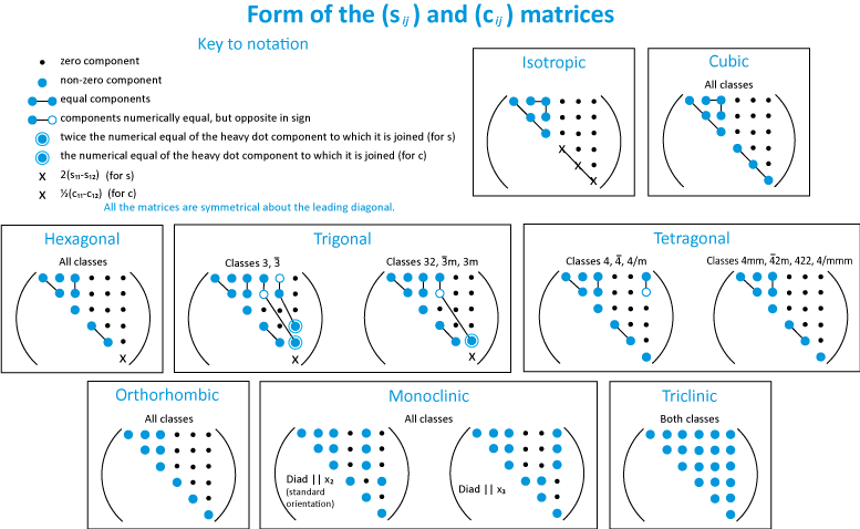
As mentioned above, the number of elastic constants needed to describe the elastic response of a crystal depends on its symmetry. Cubic crystals require three elastic constants: c₁₁,c₁₂ and c₄₄. Hexagonal crystals require five and trigonal and tetragonal crystals require six or seven depending on the point group. Orthorhombic crystals require nine constants and monoclinic crystals require thirteen. The elastic constants are affected by the state of the material including its temperature, and pressure and for minerals with solid solutions, chemical composition as well.

 

 

Additional Literature
 

 

Jaeger, J. C. Elasticity, Fracture and Flow. London: Chapman & Hall, 1969.

Jaeger, J. C.; Cook, N. G. W. Fundamentals of Rock Mechanics. London: Chapman & Hall,

1969.

Nye, J. F. Physical Properties of Crystals. London: Oxford University Press, 1959.

Bass, J.D. Elasticity of Minerals, Glasses, and Melts, Mineral Physics and Cyrstallography: A Handbook of Physical Constants, AGU Reference Shelf 2,T. J. Ahrens, Ed., American Geophysical Union, Washington DC, 1995.

Acknowledgements

These materials are being developed with the support of COMPRES, the Consortium for Materials Properties Research in Earth Sciences, under NSF Cooperative Agreement EAR 10-43050 and is partially supported by UNLV's High Pressure Science and Engineering Center, a DOE NNSA Center of Excellence supported under DOE NNSA Cooperative Agreement No. DE FC52-06NA26274.