• Formulate a standard optimization form from the problem description.
• Select an appropriate algorithm and method to solve optimization problems.
• Implement the solution using computational tools for solving optimization problems.
• Judge the feasible solutions and choose the best design for multiobjective problems
• Report the solutions in a visualized format in graphics

California State University is a four-year college with a graduate school that offers Masters degrees. The Optimum Mechanical Design is a graduate course that teaches design optimization theory and application, and MATLAB is used as a computational tool. The Global Optimization, Optimization, Partial Differential Equations, and Symbolic Math Toolboxes are used. In the Spring 2023 semester, about eight students took the course. I used a textbook, and one of the chapters of the text teaches the basics of MATLAB, focusing on the fundamentals, including using vectors and matrices. Students are assumed to have taken a MATLAB course in their undergraduate curriculum. However, many students have not used MATLAB for a while, and some have never used it before, which was one of the most significant hurdles in teaching the course. The preliminary of the course includes algebra, calculus (partial differential equations), vector and matrix computations, and fundamental MATLAB programming.
Instead of taking in-class examinations, the students must perform three small projects. The Optimal Wing Profile Design project is the second project.

The original project is from the course, "AA222/CS361: Engineering Design Optimization", offered at Stanford University. The system used Python and Julia programming languages to implement the solution.

In supersonic flight, drag forces, especially wave drag caused by shock waves, must be minimized by designing the wing's cross-section shape. Traditional aerodynamics dictates that a flat plate minimizes drag in linearized supersonic flow. However, a flat plate lacks structural integrity. Our project aims to optimize aerodynamic shapes to find alternatives that meet constraints such as minimum cross-section thickness and internal area requirements.

Aerodynamics Assumptions:

The cross-section is a 2D body, symmetrical about the x-axis, centered at (0,0), with a chord length of two units. See Figure 1 for a simplified diagram. The upper surface is approximated using 31 evenly spaced points along the x-axis, connecting the leading edge (-1,0) to the trailing edge (1,0). The z-axis position of each of these 31 points is the variable under consideration.

×

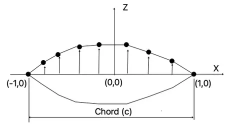Figure 1: An example airfoil geometry defined by line segments connecting 9 points. The lower surface is a mirror of the upper surface.

Reuse: This item is offered under a Creative Commons Attribution-NonCommercial-ShareAlike license http://creativecommons.org/licenses/by-nc-sa/3.0/ You may reuse this item for non-commercial purposes as long as you provide attribution and offer any derivative works under a similar license.

Aerodynamics uses the dimensionless drag coefficient to quantify the body drag force. The problem aims to minimize the coefficient for a 2D body in linearized supersonic flow. The drag coefficient (CD) calculation involves integrating the surface pressure coefficient ($C_p$) multiplied by the horizontal component of the unit average vector ($\hat{n}_x$) along the surface divided by the chord length ($c$), as shown in Equation (1).

$$C_d = \frac{1}{c} \int -C_p \hat{n}_x ds \ \ \ \ (1)$$

[code math]Given a Mach number ($M$) of 1.6, the surface pressure coefficient ($C_p$) can be expressed as a function of Mach number, as shown in Equation (2).

$$C_p = \frac{2(\frac{dz}{dx}|_{surface})}{\sqrt{M^2-1}} \ \ \ \ (2)$$

As the surface consists of line segments, Equation (1) can be transformed into a finite sum across the upper surface segments, multiplied by 2 to account for the lower surface, as described in Equation (3).

$$C_d = -\frac{2}{c}\sum_{i=1}^{30}C_{p_i}\hat{n}_{x_i}s_i \ \ \ \ (3)$$

The index variable, $i$, sums across the 30 line segments (31 points result in 30 line segments). At the same time, $C_p$, $\hat{n}_x$, and $s_i$ represent the surface pressure coefficient, the x-component of the unit normal vector, and the length of the $i_{th}$ line segment, respectively. To express Equation (3) solely as a function of $C_p$, refer to Figure 2 for a single-line segment diagram.

×

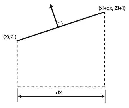Figure 2:Line segment i

Provenance: Yong Suh, California State University-Sacramento
Reuse: This item is in the public domain and maybe reused freely without restriction.

Constraints:

The cross-section of the wing must form a closed shape. To ensure this, the first and the last components of the z vector must be set to zero, aligning them with the x-axis.
For the remaining constraints, the following four different cases are considered:

• Case 1: Only the closed-body constraints described above apply, with no additional constraints.
• Case 2: A minimum thickness of 0.21 units at the center of the airfoil must be enforced in addition to the closed body constraints, specifically on the 16th component of z (z_16 >= 0.21)
• Case 3: This case enforces a fixed internal area for the airfoil and the closed body constraints, with the area set to 0.5. The inner area can be expressed as a finite sum of the area under each line segment, doubled to account for the lower surface.
• Case 4: All previously mentioned constraints must be applied in the fourth case.

What to submit:

Submit your MATLAB code and the plots of the four bodies corresponding to each case for the abovementioned four cases. Be sure to plot the upper and lower surfaces, label axes, and scale the x and z axes equally. Also, please have the grid turned on for all submitted plots. In your submission, you should also have a table that tabulates the optimal for each case with four decimal places for precision. Make any comments or observations you wish to make.

You may brainstorm ideas with other students and compare outputs, but your code must be implemented by yourself.

* Give students examples of using the MATLAB fmincon function with equality and inequality constraints. Let the students know how to add the constraints to the fmincon function.
* Tell the students what the objective function is. Show how to formulate the objective function and the constraints.
* Explain the equations and how the Cd (Equation 3) equation can be further simplified.
* Provide students with the answer drag coefficients for the four cases so that students know if their code is correct.

After finishing the assignment, students should be able to

• write basic objective-oriented programming code
• use MATLAB optimization functions such as fmincon
• implement MATLAB code of basic algorithms such as the bisection, and steepest-descend algorithms.
• MATLAB toolboxes that include symbolic math, partial differential equations, optimization, and global optimization toolboxes.
• visualize the computational result data using MATLAB 2D and 3D graphics plot functions

Solution

Objective Function

The objective function, seemingly complicated, can be simplified as follows.

$$C_d=-\frac{2}{c}\sum_{i=1}^{30}C_{p_i}\hat{n}_{x_i}s_i $$

[cde math]Substituting $C_p=\frac{(\frac{dz}{dx})}{\sqrt{M^2-1}}$[end code]

$$C_d=-\frac{2}{c}\sum_{i=1}^{30}\frac{1}{\sqrt{M^2-1}}(\frac{dz_i}{dx_i}) \hat{n}_{x_i} s_i$$

Now, $\hat{n}_{x_i} = \sin \theta$ as shown in Figure 3 below.

×

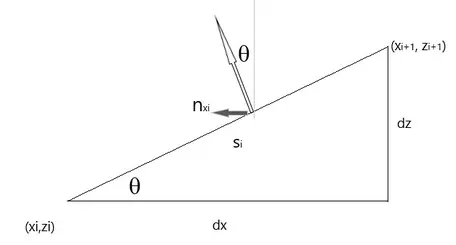Figure 3

Provenance: Yong Suh, California State University-Sacramento
Reuse: This item is in the public domain and maybe reused freely without restriction.

[code math]Also, $\sin{\theta}=\frac{dz_i}{s_i}$

Substituting,

$$C_d=-\frac{2}{c\sqrt{M^2-1}}\sum_{i=1}^{30}\frac{dz_i}{dx_i} \frac{dz_i}{s_i} s_i = -\frac{2}{c\sqrt{M^2-1}}\sum_{i=1}^{30}\frac{dz_i^2}{dx_i}$$

Create this equation as a separate MATLAB function and supply it as the first argument to the fmincon function.

Here is a source code:

%===========
% caseIn: 1, 2, 3, 4 (case 1, case 2, case 3, case 4)
%
function WingProfile(caseIn)
   if caseIn < 1 || caseIn > 
      disp("Argument values: 1 2 3 4 for each case number.");
      return
   end

   chord = 2;       % Width of the wing
   numPts = 31;   % Number of sampling points
   xArr = linspace(-chord/2, chord/2, numPts);  % Equally spaced x positions of the sampling points
   x = xArr';   % column vector
   z = [0, repelem(0.1,numPts-2), 0]';  % Arbitrary initial values in a column vector
   z0 = z;

   %=========
   % fmincon
   % X = fmincon(FUN,X0,A,B,Aeq,Beq,LB,UB,NONLCON)
   % Inequality constraints, if any
   A = []; B = [];
   % Equality constraints, if any
   Aeq = []; beq = [];
   % Lower bounds of Z
   zMin = zeros(numPts,1);
   if caseIn == 2 || caseIn == 4
      zMin(16) = 0.21; % Case 2 or case 4
   else
      zMin(16) = 0.0; % Case 1 or case 3
   end

   % Upper bounds of Z
   zMax = [0,repelem(inf,numPts-2), 0]; % start and end points: clamped at zero

   % Call fmincon
   % Case 1, 2
   if caseIn == 1 || caseIn == 2
      [z,Cd] = fmincon(@(z)coeff_drag(z,x), z0, A, B, Aeq, beq, zMin, zMax);
   % Case 3, 4
   elseif caseIn == 3 || caseIn == 4
      [z,Cd] = fmincon(@(z)coeff_drag(z,x), z0, A, B, Aeq, beq, zMin, zMax, ... @(z)areaConstraint(z,x));
   end

   % display the result
   fprintf("\nCase %d - Cd = %f\n", caseIn, Cd);
   fprintf("Max height: %f\n", max(z)); axis equal;
   plot(x,z,'*',x,-z,'*'); grid on;
   wingarea = areaWing(z,x);
   title(['Cd = ',num2str(Cd), ', Max z = ', num2str(max(z)), ', Wing area = ', num2str(wingarea)]);
   axis([-1 1 -1 1])
end

%======================================
% OBJECTIVE FUNCTION (Coefficient drag)
%
function Cd = coeff_drag(z,x)
   Cd = 0;
   con = 2/sqrt(1.6^2-1);
   for i = 1:30
      Cd = Cd + (z(i+1)-z(i))^2/((x(i+1)-x(I)));
   end
   Cd = con*Cd;
end

%======================================
% Area constraint
%
function [cineq,ceq] = areaConstraint(z,x)
   cineq = [];
   area = areaWing(z,x);
   ceq = area - 0.5;
end

function area = areaWing(z,x)
   area = 0;
   for i=1:numel(x)-1
      area = area + trapezoidArea(x(i),x(i+1),z(i),z(i+1));
   end
   area = area * 2; % upper and lower wing
end

function a = trapezoidArea(x1,x2,z1,z2);
   zmin = min(z1,z2);
   zmax = max(z1,z2);
   a = 0.5*(x2-x1)*(zmin+zmax);
end

Plots of the Wing Profiles

×

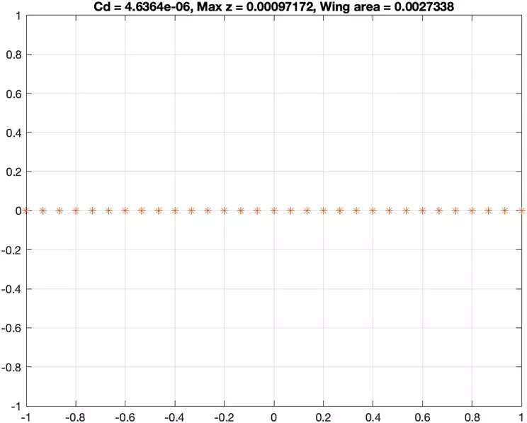Case 1: Cd=0.0000

Provenance: Yong Suh, California State University-Sacramento
Reuse: If you wish to use this item outside this site in ways that exceed fair use (see http://fairuse.stanford.edu/) you must seek permission from its creator.

×

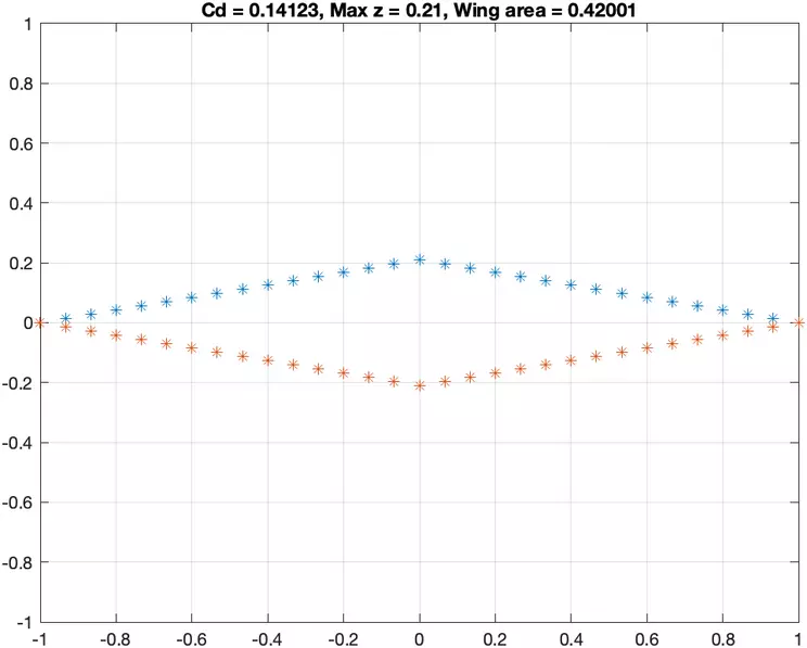Case 2: Cd=0.1412

Provenance: Yong Suh, California State University-Sacramento
Reuse: If you wish to use this item outside this site in ways that exceed fair use (see http://fairuse.stanford.edu/) you must seek permission from its creator.

×

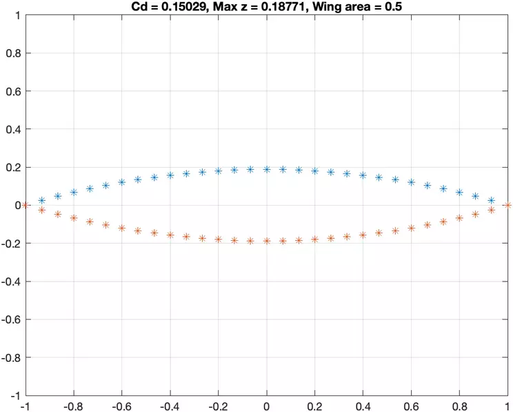Case 3: Cd = 0.1503

Provenance: Yong Suh, California State University-Sacramento
Reuse: If you wish to use this item outside this site in ways that exceed fair use (see http://fairuse.stanford.edu/) you must seek permission from its creator.

×

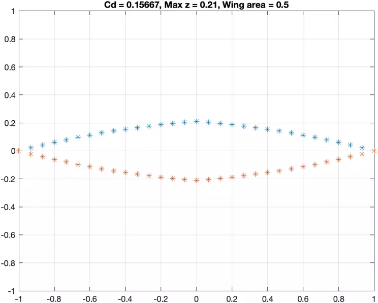Case 4: Cd = 0.1567

Provenance: Yong Suh, California State University-Sacramento
Reuse: If you wish to use this item outside this site in ways that exceed fair use (see http://fairuse.stanford.edu/) you must seek permission from its creator.

* Stanford University, AA222/CS361: Engineering Design Optimization course, Spring 2022