Initial Publication Date: August 11, 2023 | Revision: January 14, 2026
- First Publication: August 11, 2023
- Revision: April 24, 2025 -- Fixing issues uncovered during testing and review.
- Revision: May 12, 2025 -- Edits to based on testing and review.
- Revision: January 14, 2026 -- Revised for clarity and accuracy
|
Cite thisIntroductory Statistics: Practice Problems
Solving Earth Science Problems with Mean, Median, Mode, and Standard Deviation

Sedimentary layers at an outcrop.
![[creative commons]](/images/creativecommons_16.png)
Provenance: Beth Pratt-Sitaula, EarthScope Consortium
Reuse: This item is offered under a Creative Commons Attribution-NonCommercial-ShareAlike license http://creativecommons.org/licenses/by-nc-sa/3.0/ You may reuse this item for non-commercial purposes as long as you provide attribution and offer any derivative works under a similar license.
Problem 1: Bed thicknesses on an outcrop (calculating a mean)
As part of a sedimentary geology study, you need to characterize typical sedimentary bed thickness and variability. At one outcrop you measure the thickness of 8 layers. Below is the table from your field notebook. Find the mean of the measurements.
| Thickness (cm) |
| 34 |
| 39 |
| 31 |
| 33 |
| 37 |
| 32 |
| 38 |
| 33 |
Step 1. Add all the values together.
`34 + 39 + 31 + 33 + 37 + 32 + 38 + 33 = 277`
Divide the sum by the number of data points.
Step 3. Round (if necessary) and report the result, including the original units.
Since the original measurements were to the nearest cm, we round to the nearest cm: `35` cm

Hurricane Florence viewed from International Space Station in 2018, showing the eye, eyewall, and surrounding rainbands.
![[reuse info]](/images/information_16.png)
Provenance: NASA https://www.flickr.com/photos/gsfc/42828603210/
Reuse: This item is in the public domain and maybe reused freely without restriction.
Problem 2: Most common hurricane categories (find the mode)
Hurricanes are classified on a scale of 1–5 based on the Saffir-Simpson Hurricane Wind scale. A "major" hurricane is one that is a Category 3, 4, or 5.
What is the most common major hurricane type (Category 3, 4, or 5) to have made landfall in Florida since 1851?
| Florida major hurricanes |
| Name |
Saffir-Simpson Category |
Year of landfall |
| Great Middle Florida |
3 |
1851 |
| Unnamed |
3 |
1871 |
| Unnamed |
3 |
1873 |
| Unnamed |
3 |
1877 |
| Unnamed |
3 |
1882 |
| Unnamed |
3 |
1888 |
| Unnamed |
3 |
1894 |
| Unnamed |
3 |
1896 |
| Unnamed |
3 |
1906 |
| Unnamed |
3 |
1909 |
| Unnamed |
3 |
1917 |
| Unnamed |
4 |
1919 |
| Unnamed |
4 |
1926 |
| Unnamed |
4 |
1928 |
| Unnamed |
3 |
1933 |
| Unnamed |
5 |
1935 |
| Unnamed |
3 |
1944 |
| Unnamed |
4 |
1945 |
| Unnamed |
4 |
1947 |
| Unnamed |
4 |
1948 |
| Unnamed |
4 |
1949 |
| Easy |
3 |
1950 |
| King |
4 |
1950 |
| Donna |
4 |
1960 |
| Betsy |
3 |
1965 |
| Alma |
3 |
1966 |
| Eloise |
3 |
1975 |
| Elena |
3 |
1985 |
| Andrew |
5 |
1992 |
| Opal |
3 |
1995 |
| Charley |
4 |
2004 |
| Ivan |
3 |
2004 |
| Jeanne |
3 |
2004 |
| Dennis |
3 |
2005 |
| Wilma |
3 |
2005 |
| Irma |
4 |
2017 |
| Michael |
5 |
2018 |
| Ian |
5 |
2022 |
Part 1: Determine the statistic that the question is asking for.
The question asks for the most common hurricane category, so this question is asking for the mode of the hurricane category variable.
Part 2: Determine the mode in the second column (hurricane category).
Step 1: Put the hurricane category data points in order from lowest to highest.
3, 3, 3, 3, 3, 3, 3, 3, 3, 3, 3, 3, 3, 3, 3, 3, 3, 3, 3, 3, 3, 3, 3, 4, 4, 4, 4, 4, 4, 4, 4, 4, 4, 4, 5, 5, 5, 5
Step 2: Find the value that occurs the most often.
There are 23 Category 3 hurricanes, 11 Category 4 hurricanes, and 4 Category 5 hurricanes.
Here, the mode is Category 3, because there are more Category 3 hurricanes than any other in the dataset. That is, the most common type of major hurricane to make landfall in Florida since 1951 is a Category 3 hurricane.
To calculate the mode in Google Sheets or in Excel, make a column with the Saffir-Simpson Category data. Click on an empty cell and type: =MODE( ) then, move your cursor inside the parentheses. Highlight all the cells with the data, and then hit return. The mode will appear in the cell
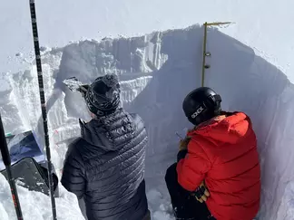
Students making observations of physical snow properties
Provenance: Robyn Gotz, Montana State University
Reuse: If you wish to use this item outside this site in ways that exceed fair use (see http://fairuse.stanford.edu/) you must seek permission from its creator.
Problem 3: Snow Water Equivalent values in the Northern Gallatin Range, Montana (calculate mean, standard deviation, median, and interpret)
Snow Water Equivalent (SWE) is a measure of precipitation derived from snow. It is the height of water per unit area if the snow were melted. An automated network of snow monitoring stations, called SNOTEL stations, record SWE in the western United States.
Below are the peak SWE values from the Lick Creek SNOTEL station in Montana for the years 2004–2023.
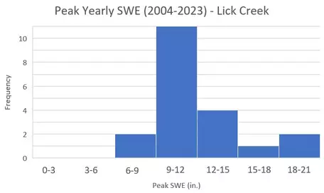
Histogram of Peak Snow Water Equivalent for the years 2004-2023 at Lick Creek
Provenance: Robyn Gotz, Montana State University
Reuse: This item is offered under a Creative Commons Attribution-NonCommercial-ShareAlike license http://creativecommons.org/licenses/by-nc-sa/3.0/ You may reuse this item for non-commercial purposes as long as you provide attribution and offer any derivative works under a similar license.
| Water Year |
Peak SWE (in.) |
| 2023 |
14.5 |
| 2022 |
11.9 |
| 2021 |
11.5 |
| 2020 |
14.2 |
| 2019 |
11.1 |
| 2018 |
15.5 |
| 2017 |
8.9 |
| 2016 |
10.5 |
| 2015 |
8.8 |
| 2014 |
18.5 |
| 2013 |
11.8 |
| 2012 |
11.0 |
| 2011 |
18.8 |
| 2010 |
10.9 |
| 2009 |
14.0 |
| 2008 |
14.1 |
| 2007 |
11.9 |
| 2006 |
10.1 |
| 2005 |
9.6 |
| 2004 |
9.9 |
Part 1: Calculate the mean peak SWE.
To calculate this in Google Sheets and Microsoft Excel: make a column with the list of SWE values. In a new cell, type: "=AVERAGE( )". Within the parentheses, highlight the list of SWE values, and hit return. The average (mean) value will be produced.
Or to do it by hand:
Step 1: Add all the values together (in this example, SWE)
`14.5 + 11.9 + 11.5 + 14.2 + 11.1 + 15.5 + 8.9 + 10.5 + 8.8 + 18.5 + 11.8 + 11.0 + 18.8 + 10.9 + 14.0 + 14.1 + 11.9 + 10.1 + 9.6 + 9.9 = 247.5` in
Step 2: Divide the sum by the number of data points.
The sum is calculated in Step 1 and there are 20 measurements, so the mean is `247.5 /20=12.375` in
Step 3: Round (if necessary) and report the result, including the original units.
Since the data are measured to a tenth of an inch, round to that and include units: 12.4 in.
Part 2: Calculate the standard deviation of the SWE data.
To calculate this in Google Sheets and Microsoft Excel: In a new cell, type: "=STDEV( )". Place your cursor within the parentheses, highlight the list of SWE values, and hit return. The standard deviation value will be produced.
This is seldom done by hand, as it is simpler and avoids errors to use Sheets or Excel.
Standard deviation `= sqrt(((value1-mean)^2+(value2-mean)+(value3-mean)+etc)/(n - 1)`
Step 1. Determine the mean of the data values.
This was done above. Mean SWE = 12.4 in.
Step 2. Calculate the square of the difference from the mean for each data value.
Make a table of the values, determine the difference to the mean from each value, and then square the differences.
`(value-mean)^2`
| Water Year |
Peak SWE (in) |
Difference from mean |
Square of difference from mean |
| 2023 |
14.5 |
2.13 |
4.5156 |
| 2022 |
11.9 |
-0.48 |
0.2256 |
| 2021 |
11.5 |
-0.88 |
0.7656 |
| 2020 |
14.2 |
1.83 |
3.3306 |
| 2019 |
11.1 |
-1.28 |
1.6256 |
| 2018 |
15.5 |
3.13 |
9.7656 |
| 2017 |
8.9 |
-3.48 |
12.0756 |
| 2016 |
10.5 |
-1.88 |
3.5156 |
| 2015 |
8.8 |
-3.58 |
12.7806 |
| 2014 |
18.5 |
6.13 |
37.5156 |
| 2013 |
11.8 |
-0.57 |
0.3306 |
| 2012 |
11.0 |
-1.38 |
1.8906 |
| 2011 |
18.8 |
6.43 |
41.2806 |
| 2010 |
10.9 |
-1.48 |
2.1756 |
| 2009 |
14.0 |
1.63 |
2.6406 |
| 2008 |
14.1 |
1.73 |
2.9756 |
| 2007 |
11.9 |
-0.48 |
0.2256 |
| 2006 |
10.1 |
-2.28 |
5.1756 |
| 2005 |
9.6 |
-2.78 |
7.7006 |
| 2004 |
9.9 |
-2.48 |
6.1256 |
Step 3. Add all the squared differences obtained in Step 2.
`4.5156 + 0.2256 + 0.7656 + 3.3306 + 1.6256 + 9.7656 + 12.0756 + 3.5156 + 12.7806 + 37.5156 + 0.3306 + 1.8906 + 41.2806`
` + 2.1756 + 2.6406 + 2.9756 + 0.2256 + 5.1756 + 7.7006 + 6.1256 = 156.6375`
Step 4. Divide the sum of the squared differences (from Step 3) by the number of data points minus 1.
Step 5. Take the square root of the result you obtained in Step 4.
Step 6. Round (if necessary) and report the result, including the original units.
Since the data are measured to a tenth of an inch, round to that and include units: s = 2.9 in.
Part 3: Calculate the median SWE.
To calculate this in Google Sheets and Microsoft Excel: In a new cell, type: "=MEDIAN( )". Place your cursor within the parentheses, highlight the list of SWE values, and hit return. The median value will be produced.
Or to do it by hand:
Step 1: Order the values from lowest to highest.
8.8, 8.9, 9.6, 9.9, 10.1, 10.5, 10.9, 11.0, 11.1, 11.5, 11.8, 11.9, 11.9, 14.0, 14.1, 14.2, 14.5, 15.5, 18.5, 18.8 in
Step 2: Find the value in the center of the ordered values.
Because there are 20 values, the middle is between values #10 (11.5) and #11 (11.8). Take the average of those two values
`(11.5 + 11.8)/2` to get the median.
Median = 11.65 in
Part 4: Interpret your findings. What does the standard deviation tell us about the spread of the SWE data? Would mean or median be a better measure of the central tendency of the SWE data?
The standard deviation of the SWE data is 2.8 in, which is fairly small compared to both the mean (12.4 in) and the median (11.7 in). This shows that the data points are generally close together and that variability in SWE over the 20 years from 2004 to 2023 is low.
Histogram of Peak Snow Water Equivalent for the years 2004-2023 at Lick Creek
Provenance: Robyn Gotz, Montana State University
Reuse: This item is offered under a Creative Commons Attribution-NonCommercial-ShareAlike license http://creativecommons.org/licenses/by-nc-sa/3.0/ You may reuse this item for non-commercial purposes as long as you provide attribution and offer any derivative works under a similar license.
When considering whether mean or median is a better measure of the central point of the data, it would be best to graph the distribution of the data in a
histogram and see if it looks like a normal distribution (with a classic bell-shaped curve). Mean and standard deviation are appropriate to use with normal distributions, while medians are appropriate for skewed or bimodal data. The histogram is shown here. It does not show a normal distribution and is slightly
right-skewed. This suggests we probably want to use median instead of the mean to describe this data. The mean (12.4 in) is slightly higher than the median and thus does not lie in the center of the data points.

Provenance: NSIDC https://www.flickr.com/photos/nsidc/51845311960
Reuse: This item is offered under a Creative Commons Attribution-NonCommercial-ShareAlike license http://creativecommons.org/licenses/by-nc-sa/3.0/ You may reuse this item for non-commercial purposes as long as you provide attribution and offer any derivative works under a similar license.
Problem 4: Permafrost thaw (calculate mean, standard deviation, median, and interpret)
Permafrost thaw is an issue of great concern in the arctic and subarctic regions of the world. The uppermost layer of soil, called the "active layer," thaws in the summers, but the permafrost below stays frozen. The thickness of the active layer has been increasing with climate warming, as more permafrost thaws and becomes part of the active layer.
Your job is to monitor the depth of the active layer at a monitoring plot. The plot (100 m x 100 m) contains 12 measurement sites equipped with frost tubes and soil temperature cables. During peak summer each year, you obtain measurements of the thickness of the active layer to add to a long-term dataset. Your values for the active layer thicknesses at the plot in the most recent year are as follows.
| Site |
Active layer thickness (cm) |
| 1 |
30 |
| 2 |
45 |
| 3 |
120 |
| 4 |
25 |
| 5 |
63 |
| 6 |
12 |
| 7 |
54 |
| 8 |
68 |
| 9 |
55 |
| 10 |
39 |
| 11 |
46 |
| 12 |
67 |
Part 1: Calculate the mean of the data.
To calculate the mean in Sheets or Excel: make a column of the active layer thickness data. Click on an empty cell and type: =AVERAGE( ). Then, move your cursor inside the parentheses. Highlight all the cells with the data, and hit return. The mean will appear in the cell.
Final step: Round (if necessary) and report the result, including the original units.
Since the measurements are made to the nearest centimeter, no rounding is needed. The answer is 52 cm.
Part 2: Calculate the standard deviation.
To calculate the standard deviation in Sheets or Excel: In a new cell, type: "=STDEV( )". Place your cursor within the parentheses, highlight the list of active layer thickness values, and hit return. The standard deviation value will be produced.
Final step: Round (if necessary) and report the result, including the original units.
The data is in centimeters, so round to the nearest whole centimeter.
s = 27 cm
That is, most of the data fall within 27 cm of the mean value of 52 cm
Part 3: Calculate the median of the data
To calculate the median in Sheets or Excel: In a new cell, type: "=MEDIAN( )". Place your cursor within the parentheses, highlight the list of active layer thickness values, and hit return. The median value will be produced.
The median thickness of the active layer is 50 cm
Part 4: Which is a more appropriate statistic for the active layer data, mean or median?
Answer:
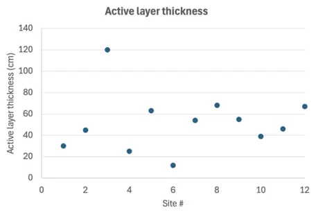
Plotting the permafrost active layer thicknesses at the different sites makes it easier to see the outlier.
Provenance: Beth Pratt-Sitaula, EarthScope Consortium
Reuse: This item is offered under a Creative Commons Attribution-NonCommercial-ShareAlike license http://creativecommons.org/licenses/by-nc-sa/3.0/ You may reuse this item for non-commercial purposes as long as you provide attribution and offer any derivative works under a similar license.
Here, we have a small dataset with one very noticeable outlier (120 cm). We know that data sets with outliers are better described using the median as a measure of the central tendency of the data. Surprisingly, the mean and median for this data set are very similar. This happened by chance, and we would not expect that to be true of all datasets with outliers. So, using the median would be the best for the permafrost data.
Next Steps
TAKE THE QUIZ!!
I think I'm competent with introductory statistics and I am ready to take the quiz! This link takes you to WAMAP. If your instructor has not given you instructions about WAMAP, you may not have to take the quiz.Or you can go back to the Introductory Statistics explanation page.