Part 2: Use ImageJ to Analyze How the Sea Ice Extent in the Arctic Has Changed Over Time¹ ²

Polar Peril

Minimum Sea Ice Extent - September

Sea ice - frozen, floating sea water - forms and melts with the seasons. If the ice grows thick enough, it does not melt completely, persisting from year to year. In the Arctic, the area covered by sea ice typically shrinks in the summer and expands in the winter.

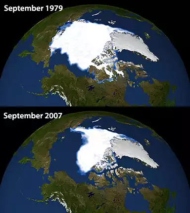
Since the late 1970s, satellite data from NASA's Nimbus 7 satellite and the Defense Meteorological Satellite Program's SSMI (Special Sensor Microwave Imager) have shown that the average area, or extent, of Arctic sea ice remaining at the end of the summer melt has decreased dramatically, falling by over 8 percent per decade. In September 2007, the sea ice extent was at a record low.

The decrease in Arctic sea ice has widespread and significant environmental impacts, particularly on animal life. Dr. Claire Parkinson, a scientist at NASA's Goddard Space Flight Center, Greenbelt, Md., and Ian Stirling, a senior scientist with the Canadian Wildlife Service, Edmonton, Alberta, used the satellite data to study sea ice coverage in areas with significant polar bear populations. In most of these areas, they found the summer melt occurring 7 to 8 days earlier each decade. Not only is the sea ice melting earlier each year, it is also returning later in the fall. This combination of early melt and late freeze has created a longer open water season and some hungry polar bears!

Polar bears hunt seals and other marine mammals on winter sea ice and fast on land during the summer melt. As the summer melt occurs earlier and earlier, the balance between the bears' feeding and fasting seasons is shifting. During the summer months the bears are forced to retreat to land and fast on their stored fat reserves until sea ice comes back in the fall. This has caused the average weight of female polar bears to fall by nearly 150 lbs. over the past 25 years. As females become lighter, their ability to reproduce and the survival of their young declines. Hungry bears are more likely to adapt to new habitats and move closer to human settlements as they seek food. This often gives the false impression that the polar bear population is actually increasing.

Investigation question:

How has the sea ice extent in the Arctic changed over time?

Download the Sea Ice Data

Right click (Win) or control-click (Mac) the link below to download the november_arctic_sea_ice.tif stack to your Day 5 directory or folder.
november_arctic_sea_ice.tif (TIFF 3.9MB Jan23 10)

Launch ImageJ; Open and Explore the Stack

Canada's Hudson Bay was chosen for this investigation because it is an important polar bear habitat. The return of the sea ice to the bay is an important event in the lives of the bears, representing the end of their fasting season. November was chosen as a key indicator month for studying the return of ice to the region.

Launch ImageJ by double-clicking its icon on your desktop or by clicking its icon in the dock (Mac) or Launch Bar (Win).
Choose File > Open, navigate to your Day 5 directory or folder, and open the november_arctic_sea_ice.tif stack.
To animate the stack and observe the changing extent of sea ice, choose Image > Stacks > Tools > Start Animation. Slow down the animation by choosing Image > Stacks > Tools > Animation Options... and set the speed to 5 frames per second. You may wish to experiment with other speeds.
Move through the stack frame by frame to carefully explore the stack. First, click on the stack to stop to stop the animation. Then drag the scroll bar at the bottom of the stack window to the right and left to scroll forward and backward through the stack. You can also use the Next Slice (>) and Previous Slice ( keyboard shortcuts to move forward and backward through the stack.

Show me the location of the scroll bar

The Sea Ice Stack shows a gradual change from blue (0% ice) to white (100% ice). Land areas are shown in green and coastlines are outlined in black.

The grey "hole" in the middle of the image is not open water, it's "missing" data. Between 1978 and the present, two different satellites — in different orbits and with different sensors — were used to gather the sea ice data. The sensors' characteristics differ slightly, most notably in how near to the pole they can obtain data. The older sensor was not able to collect data north of 83 degrees latitude; the newer one can obtain data as far north as 87 degrees latitude. Thus, the "hole" appears to get smaller at some point in time.

This missing data is not a real problem, because we can reasonably assume that any region north of 83 degrees latitude is covered with ice throughout the year. Thus, we can assume that the "pole hole" where the sensors do not obtain data is "ice-covered." This allows extent estimates to be continuous over the whole record.

Measure the Sea Ice Extent

In order to make area measurements in real world units — in this case, square kilometers — set a spatial scale for the image. Choose Analyze > Set Scale. The Set Scale window opens. Set the Distance in Pixels to 1, the Known Distance to 25, and the Unit of Length to km.

Show me the Set Scale window

To measure the extent of the sea ice — defined as areas covered by at least 15% ice — you'll need to Threshold the image to select only those pixels with concentrations of ice from 15-100%. Thresholding selects and highlights in red all of the pixels in the image that are within a specific range of values.
- Choose Image > Adjust > Threshold.
- Pixels that have values between 38 (15% ice) and 250 (100% ice) represent ice covered pixels. Threshold the image to highlight values from 38 to 251. By using 251 instead of 250, you also select the pole hole region.
- Do NOT click Apply or anything else in the Threshold window; simply close the Threshold window.
Show me the steps to adjust the threshold

Hide
- Choose Image > Adjust > Threshold.
- The Threshold window opens. Threshold the image to highlight values from 38 to 251. Drag the lower threshold limit to 38.
- Drag the upper threshold limit to 251.
Show me a movie on how to adjust the threshold range

Hide
Drag the sliders to set the lower threshold limit to 38 and the upper threshold limit to 251.
Next, select the thresholded area. Use the Magnifying Glass tool to zoom in on Hudson Bay. Then use the Polygon Selection tool to select Hudson Bay.

Show me the steps to select Hudson Bay

Show me a movie about how to select Hudson Bay

Use the Magnifying glass tool

to zoom in on Hudson Bay, then use the Polygon selection tool

to outline Hudson Bay. Click the tool each time you want to create a vertex (turn) in the line. To complete the selection, click in the small box that appears at the beginning of the selection line.

Choose Analyze > Set Measurements and turn on the Area, Stack Position, and Limit to Threshold options. All other options should be turned off.

Show me how to set measurements

Start at slice 1 and choose Analyze > Measure to measure the area of the highlighted pixels within the selected area. Choose Image > Stacks > Next Slice to advance to the next slice. Measure the next slice, and repeat until all 30 slices are measured.

Show me how to measure the slices of a stack

Start at slice 1 and choose Analyze > Measure to measure the area of the highlighted pixels within the selected area.
The Results window opens. Your measurement should be similar to this one.
Choose Image > Stacks > Next Slice to advance to the next slice. Measure the next slice, and repeat until all 30 slices are measured. When you are finished, the Results window will display all your measurements.