Dimensional Analysis and Flow Visualization Using MATLAB
Summary
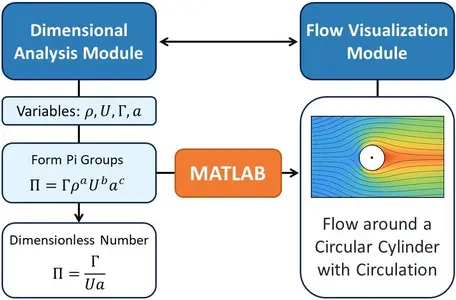
In this MATLAB-based activity, students develop two general computational modules, one for automated dimensional analysis using the Buckingham π theorem, and another for streamline and pathline visualization for arbitrary velocity fields. These tools are designed to be reusable across a range of physical and engineering systems. Once validated on classical benchmark problems, the modules are applied to a capstone problem: the potential flow around a circular cylinder with circulation. Through this workflow, students connect the abstract principles of scaling and similarity to the tangible visualization of flow dynamics, building an integrated understanding of computational, analytical, and physical reasoning.
![[creative commons]](/images/creativecommons_16.png)
Learning Goals
By completing this activity, students will be able to:
- Automate dimensional analysis through MATLAB by constructing a rank-based algorithm for the Buckingham π theorem.
- Develop general computational tools for streamline and pathline visualization applicable to arbitrary velocity fields.
- Validate and test their algorithms using canonical benchmark problems with known analytical results.
- Apply their tools to analyze the nondimensional parameters and flow structures of potential flow around a circular cylinder with circulation.
- Strengthen their ability to connect mathematical formulation, numerical implementation, and physical interpretation.
- Reflect on the computational process by evaluating assumptions, interpreting limitations of their models, and identifying how their approach could be improved/extended.
Context for Use
This activity is appropriate for undergraduate-level Fluid Mechanics and/or Introduction to Computational Methods in Engineering, and it is best suited for an extended 2–3 week project (or shorter if simplified). The activity can be completed as a group project or an individual assignment. Students should have prior exposure to:
- Buckingham π theorem and basic dimensional analysis,
- fluid kinematics and potential flow concepts, and
- MATLAB fundamentals (symbolic math, plotting, array operations).
Description and Teaching Materials
Part 1: Dimensional Analysis Module: Students build a MATLAB application or Live Script that automatically identifies independent dimensionless groups for any given set of variables. In particular, they:
- Input variable names and their fundamental dimensions (M, L, T).
- Construct the dimensional matrix and compute its rank.
- Determine the number of independent π groups and their symbolic forms using the null space of the dimensional matrix.
- Implement checks to ensure user-selected repeating variables are dimensionally independent.
- Display the resulting π groups and their physical meaning in tabular and symbolic form.
- The tool is validated using known examples such as the pendulum period, drag on a sphere, open-channel flow, and capillary wave speed.
Part 2: Streamline and Pathline Visualization Module: Students then develop a MATLAB app, Live Script, or modular function capable of generating streamlines and pathlines for any two-dimensional velocity field (steady or unsteady). This module emphasizes algorithmic structure, visualization quality, and the physical interpretation of flowlines. They:
- Allow user-defined analytical velocity components or imported data.
- Numerically integrate the streamline equations and the pathline ODEs using solvers like ode45.
- Implement visualization options, including colored trajectories, arrows, and overlays of multiple seed points.
- Validate their module using canonical flows such as uniform flow, solid-body rotation, stagnation point flow, point vortex, and unsteady shear flow.
Part 3: Potential Flow Around a Circular Cylinder: Finally, students integrate both modules to analyze potential flow around a circular cylinder with circulation, modeled as the superposition of a uniform flow, a doublet, and a point vortex. They:
- Use the dimensional analysis tool to identify the governing nondimensional parameters (e.g., Re = ρUL⁄μ and Γ⁄Ua).
- Use the flowline module to compute and visualize nondimensional streamlines and pathlines.
- Perform parameter studies for different circulation ratios and discuss flow symmetry, stagnation points, and implied lift.
- Present results as nondimensional contour plots and interpret trends in their report.
Teaching Notes and Tips
Below are some general teaching notes and tips:
- Begin with a short review lecture on dimensional analysis and potential flow theory before introducing the computational task.
- Encourage group work (2–3 students) for code development and discussion.
- Scaffold the project by providing a basic MATLAB framework or pseudocode for flow visualization; let students expand functionality.
- For novice programmers, Live Scripts are ideal for incremental testing and visualization.
- Optionally, you can include experimental data comparison. In this case, ensure datasets are scaled and cleaned (e.g., CSV or MAT format).
Assessment
Formative Assessment: Formative assessment takes place throughout the activity as students engage in guided coding sessions (with a TA), peer discussions, and instructor-led debugging. During these checkpoints, students receive targeted feedback on their code implementation, visualization accuracy, and dimensional reasoning. Code reviews emphasize structure, readability, and correctness, ensuring that each student can effectively translate physical models into computational algorithms. These formative exercises help instructors identify misconceptions early and allow students to iteratively refine their understanding of flow behavior and nondimensional scaling before final submission.
In addition, during coding milestones and validation checkpoints, students submit a brief (1–2 paragraph) reflective statement summarizing what they learned, the challenges they encountered, and how their approach evolved. These reflections provide instructors with insight into each student's problem-solving process and help ensure that conceptual understanding develops in parallel with computational proficiency.
Summative Assessment: For summative assessment, students submit a comprehensive MATLAB report and code package that includes plots, well-commented scripts, and an explanation of how nondimensional parameters influence the resulting flow patterns. In addition, they write a 1-2 page reflection discussing the physical meaning of the derived dimensionless groups, the observed changes in flow topology (e.g., stagnation points and circulation effects), and, if applicable, a comparison between their computational predictions and experimental data (optional). This combination of quantitative coding evaluation and qualitative interpretation ensures that students demonstrate both computational competency and conceptual fluency in applying MATLAB to fluid mechanics. In addition, the report must include a short reflection section in which students discuss what they learned through developing and applying their MATLAB modules. They should consider:
- What did they find most challenging about translating physical concepts into computational form?
- How did the dimensional analysis or flow visualization tools change their understanding of the underlying fluid mechanics?
- If they had more time, what improvements or extensions would they pursue?
Rubric for MATLAB Report: rubric.pdf (Acrobat (PDF) 149kB Oct27 25)
References and Resources
- White, F.M. (2016). Fluid Mechanics, 8th Ed. McGraw-Hill Education.
- Kundu, P.K., Cohen, I.M., & Dowling, D.R. (2015). Fluid Mechanics, 6th Ed. Academic Press.