Unit 2: Global Sea-Level Response to Temperature Changes: Temperature and Altimetry Data

Unit 2 Learning Outcomes

×

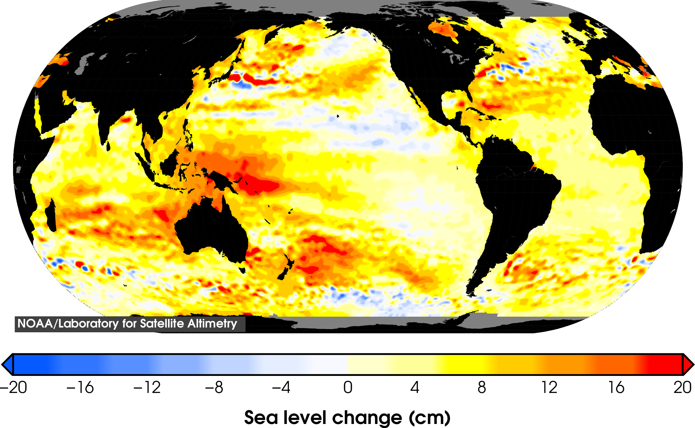
Total sea level change since 1993. In this unit, students will asses the contribution of seawater thermal expansion to sea level rise, as shown in this image. Image from NOAA

Provenance: Source: https://www.star.nesdis.noaa.gov/sod/lsa/SeaLevelRise/slr/mssh_2014-1993_300.png
Reuse: This item is offered under a Creative Commons Attribution-NonCommercial-ShareAlike license http://creativecommons.org/licenses/by-nc-sa/3.0/ You may reuse this item for non-commercial purposes as long as you provide attribution and offer any derivative works under a similar license.

Students will be able to:

• Create time-series plots of sea surface temperature and assess recent sea surface temperature change.
• Calculate how much sea-level rise has occurred due to thermal expansion of the oceans.
• Contrast observed sea-level rise data with the calculated sea-level rise due to thermal expansion and determine how much observed sea-level rise is attributable to thermal expansion.
• Propose additional sources of sea-level rise.

Show More info on how learning outcomes connect to science literacy principles and module goals

Hide

Unit 2 Teaching Objectives

• Cognitive: Enable students to demonstrate the connection between changes in sea surface temperatures and the processes that result in changes in sea level.
• Behavioral: Promote skills in making and interpreting graphs, and using linear equations to calculate sea surface temperature changes over time.
• Affective: Facilitate the students' appreciation that numerous processes must be considered when assessing the causes of sea-level rise.

The content in Unit 2 is appropriate for advanced Climate, Cryosphere, Geology, Geoscience, or Environmental-related courses conducted at the junior and/or senior level in which geodesy data can be introduced. Students should be cognizant that the Earth's climate is warming and have familiarity with the causes of the warming. The student exercise in Unit 2 requires access to computers to create Excel (or similar) graphs and calculations, so the exercise is best executed in a computer lab setting or could be assigned as an out-of-class activity. Students will need basic proficiency in creating graphs from time-series data sets, including conducting linear trend analysis. Unit 2 is designed to follow Unit 1: Climate Change and Sea Level: Who Are the Stakeholders?, in which students consider affected stakeholders in a vulnerable coastal region. Some preparatory lecture time may be required to introduce the concept of thermal expansion and the measurement of sea level using satellite radar altimetry. Following completion of the student exercise, there is additional material that could be covered in class on causes of sea-level rise in addition to thermal expansion. If the entire two-week module will not be utilized, we recommend pairing Unit 2 with Unit 3: Global Sea Level Response to Ice-Mass Loss: GRACE and InSAR data to give students an opportunity to investigate the dominant causes of current sea level.

Introduction

In this unit, students work through an exercise with sea surface temperature and radar-derived sea-level data. The student exercise takes 1–3 hours (depending on students' familiarity with working with spreadsheets and creating graphs) that could be done in a lab period, stretched across several shorter class periods, or done partly/largely as a homework assignment.

Three PowerPoint presentations provide background information relevant to this unit. The first reviews the basics of thermal expansion, and includes a slide that shows that the majority of additional energy in the Earth's climate system is stored in the oceans. The second presentation provides an overview of satellite radar altimetry and its use to measure global sea level. This information should be reviewed prior to students working on the Unit 2 student exercise. The third presentation is a tutorial that walks students through using Excel to plot data, add trend lines and linear fits, and how to use the equation of the line to calculate rates of change.

Student Exercise Elements

The Unit 2 student exercise requires that students have access to a computer and Excel (or similar). Students can complete the Unit 2 student exercise either during class or lab time, or as a take-home activity. In Part 1 of the student exercise, students create graphs of historical (1880–2015) sea surface temperature (SST) data and evaluate how much SST has increased historically and during the period of overlap with the satellite radar altimetry data (1993–2015). In Part 2, students use the sea surface temperature data to calculate how much sea-level rise would have occurred during 1993–2015 due to thermal expansion. In Part 3, students compare observed sea-level rise to their calculations of sea-level rise due to thermal expansion and consider additional sources of sea-level rise. This exercise is best completed individually.

Discussion to Follow the Exercise

A small group or class discussion can follow completion of the student exercise based on Question 10 from the student exercise: What other sources may be contributing to sea-level rise besides thermal expansion? Students can brainstorm. A PowerPoint presentation provides information on additional sources of sea-level rise and demonstrates that thermal expansion is the largest source of sea-level rise (based on the 1993–2010 time period).

Following the discussion, instructors may want to assign the students to read Nerem et al. (2018) Climate-change–driven accelerated sea-level rise detected in the altimeter era. This short article addresses additional causes of variability in the sea-level satellite radar altimetry data, including volcanic eruptions, El Niño Southern Oscillation, and potential errors in the data due to instrument drift, and demonstrates that the rate of sea-level rise is accelerating.

Teaching Materials

• Presentations
  • Overview of Thermal Expansion (PowerPoint 2007 (.pptx) 2MB Nov8 19)
    
    
    Click to view
    
    
  • Overview of Satellite Radar Altimetry (PowerPoint 2007 (.pptx) 226.3MB Nov13 19)
    
    
    Click to view
    
    
  • Excel tutorial for creating trend lines and calculating rates of change (PowerPoint 2007 (.pptx) 1.9MB Nov8 19)
    
    
    Click to view
    
    
• Student Exercise Files
  • Exercise: Unit 2 Student Exercise Sea Level and Temperature (Microsoft Word 2007 (.docx) 409kB Apr19 21) PDF (Acrobat (PDF) 432kB Apr19 21)
  • Data set: Unit 2 Student Exercise Data File (Excel 2007 (.xlsx) 36kB Apr19 21)
• Student Exercise Answer Keys
  • Exercise:
    Unit 2 Student Exercise Answer Key -- private instructor-only file
    Hide
    Unit 2 Student Exercise Answer Key

    
    This file is only accessible to verified educators. If you are a teacher or faculty member and would like access to this file please enter your email address to be verified as belonging to an educator.

    Email Adress Submit

  • Data set:
    Unit 2 Student Exercise Data File Instructor Calculations -- private instructor-only file
    Hide
    Unit 2 Student Exercise Data File Instructor Calculations

    
    This file is only accessible to verified educators. If you are a teacher or faculty member and would like access to this file please enter your email address to be verified as belonging to an educator.

    Email Adress Submit

• Supplementary slides for the class discussion
  • Unit 2 Sources of Sea Level Rise (PowerPoint 2007 (.pptx) 2.8MB Nov8 19)
  • 
    Click to view
    
    
• Optional follow-up reading for further discussion: Nerem et al. (2018) Climate-change–driven accelerated sea-level rise detected in the altimeter era

• The unit requires use of computers. Ideally each student will have their own computer or laptop. At least there should be one computer per work group. If it is not feasible to use computers during the class/lab period, the instructor should take extra steps to make sure that students understand what is required of them to do the exercise outside of class.
• The sea surface temperature data in the module are presented as temperature anomalies, rather than average temperatures. The anomalies used here are calculated based on the average temperature during 1971–2000. Anomalies are of course very commonly used in climate studies as a way to easily compare changes observed in different places rather than compare the specific temperature (or other parameter). This unit does not spend much time explaining anomalies, under the assumption that most majors-level students will have encountered the concept before. If, however, this idea is new for your students, you may want to spend a bit more time introducing them to the definition and function. Example resources on Anomalies vs Temperature.
• The provided data files are in Excel. Students may actually prefer to use another spreadsheet program such as Google Sheets if they are working on their own computers. Google Sheets, while less powerful than Excel, has the capabilities to do the analyses for this unit. The Excel files should open fine in Sheets, but you may want to double-check this process yourself if you are not familiar with it. If you have students working on their own computers and thus have different software and different versions, it is better to emphasize the processes and how to query Help rather than try to show exactly the on-screen steps for the different programs.
• Although the x-intercept values are not emphasized in the exercise (slope being much more important), students may find them confusing when they plot the equation of the line on a scatter plot. The x-intercept in this case is referencing back to 0 A.D., which is of course, not very relevant to the exercise. An alternative is to make the plots using a line graph option. In this case, the equation of the linear trend line will have an x-intercept value at the first year of the interval time period. A worked example of this is in the instructor answer key version of the data spreadsheet.
• There are several different ways that students may approach calculating increases in Annual SST anomalies in Question 2. The instructor should be prepared for a range of answers, or provide guidelines for the specific approach the instructor wants the students to use.
• If this unit is completed in class and there are students with less experience working with Excel (or similar), the instructor may want to have more experienced students help the more novice students.
• For students not familiar with the role of thermal expansion in sea-level rise, this unit is very informative to show the large contribution of thermal expansion to sea-level rise.
• The Teaching with Spreadsheets across the Curriculum site provides support for teaching with programs such as Excel. If your students need supporting math practice, The Math You Need site provides an opportunity to brush up on skills such as graphing and unit conversion.
• If students will be completing the Stakeholder Report in Unit 5, it is useful for the instructor to remind the students that they can be incrementally working on Unit 5 by beginning to incorporate their findings from Units 1 and 2.

Formative assessment of student learning may be done through conversations with individuals and groups during the exercise if it is done during class time. The student exercise is the summative assessment for the unit. The Unit 2 Assessment Rubric (Microsoft Word 2007 (.docx) 19kB Nov12 19) PDF (Acrobat (PDF) 65kB Nov12 19) provides an example of how the exercise can be evaluated. We suggest including the rubric with the student exercise so the students know the criteria ahead of time. The discussion provides a less formal form of summative assessment and is also helpful for encouraging student reflection.

• Information on the thermal expansion rate given in this unit (100 mm/1oC) was extrapolated from information in the report IPCC Climate Change 2014: Impacts, Adaptation, and Vulnerability.
  Assumed change in sea level due to thermal expansion accounts for 30 to 55% (average 42.5%) of twenty-first-century global mean sea-level rise in the Representative Concentration Pathways (RCPs) projections (IPCC 2014). For example, the likely range in global mean sea-level rise for the RCP2.6 scenario is 170 mm to 320 mm with a mean of 240 mm, for a temperature increase of 1oC. The average of the thermal expansion values is 42.5%. This gives us 100.8 mm (42.5 % of 400 mm) sea-level rise for 1oC temperature increase. On the other hand, if we are to consider the average thermal expansion of the lower limit (170 mm) and upper limit (320 mm), we get 40.8 mm/oC and 134.4 mm/oC, respectively. We can also calculate other scenarios using the lower and upper limit of thermal expansion itself, however the average value of 100 mm has the added benefit of being easy to use in calculations. In general, thermal expansion hovers around similar values for the other RCPs. The largest contribution to global mean sea level is coming from melting glaciers.
• The University of Colorado Sea Level Group website provides up-to-date global mean sea-level time series in addition to a wide range of other related data sets (regional sea level, tide gauge sea level) and other web resources related to sea level (see their Sea Level Links).
• This Radar Altimetry Tutorial and Toolbox by the European Space Agency (ESA) provides detailed information about satellite radar altimetry.
• UNAVCO tutorials provide additional information about GPS/GNSS, ellipsoids, and geoids