Part 2—Import, Animate, and Measure Sea Ice
Step 1 – Launch ImageJ and Import the Sea Ice Data


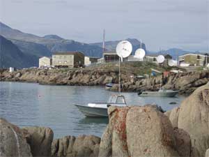
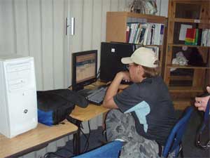
Thanks to an efficient satellite connection to the Internet (and some nimble students), the team downloads the sea ice images to their local computers. They animate the images to show the changes in seasonal sea ice extents over the past 30 years and excitedly share what they see in the changing "seasons of ice." The elders in their village have said that in recent years, the ice is leaving earlier each spring and returning later each fall. The satellite images they see on their computers confirm native knowledge!
- Launch ImageJ by double-clicking its icon
 on your desktop (Mac or PC) or by clicking the icon in the dock (Mac) or the Start menu (PC).
 - From ImageJ's main menu choose File > Import > Raw, then navigate (browse) down inside the folder of data until you see the monthly folder.
- Click once on the first file in the folder to select it, then click Open.
- In the dialog box that appears, set the fields as shown in the image below.

Some notes about importing sea-ice data sequences:
- If you choose to explore sea ice images for the Southern Hemisphere, use a width of 316 pixels and a height of 448 pixels
- All fields to be imported must be in the same directory or folder.
- File names for the fields should be such that they are imported into ImageJ in the appropriate order: ImageJ reads in by alphanumeric order, so to import sequentially by time, the file names should have YYYYMMDD order for the date.
- Click OK and wait for ImageJ to import all 333 fields. This is a large amount of data so it may take a minute or so.
- Save your stack by choosing File > Save As > Tiff... from ImageJ's menu bar. Name it sea-ice_extents.tif
Step 2 – Apply a Color Scale (Look-Up Table) to the Images
The fields will come in as grayscale images. Adding a color scale that differentiates between ice and water will help you visualize the extent of the sea ice. To begin, you will download and apply a color scale (also called a look-up table or LUT) prepared by Dr. Walt Meier.
- Right-click (control-click on a Mac) on the link below and select the "Save link as..." option from the pulldown menu. Save the file to your Sea Ice folder or directory as a .txt file.
Sea Ice Look Up Table (LUT) (Text File 4kB Jun21 07) Note: if this link opens into your browser, click your Back button and try again. You need to download the file to your own computer to use it. - In ImageJ, select File > Import > LUT and navigate to where you saved the LUT file. Select the file and click open.
Step 3 – Animate the Images
To get an overview of monthly sea ice changes, you will animate this stack of 333 satellite images to make a mini movie. This will allow you to review nearly 20 years of data in a matter of minutes. Enjoy the show!
- In ImageJ, start the animation by choosing Image > Stacks > Tools > Start Animation.
- Image > Stacks > Tools > Stop Animation stops the animation.
- Use Animation Options under the same pulldown menu as the start and stop animation, to control the speed, or use the "." and "," keys on your keyboard to move forward or back one frame at a time.
- You could also choose to have the stack tools (see below for screen shot of stack tools) show up in the Image J toolbar. This will give you a controller for your animation.
- Watch the movie carefully enough to get a sense of the changes in sea ice over a single year. You can look at the file names in the upper left corner of the window to see what month is being displayed. Consider the following questions:
- What happens to sea ice over a year?
- What month would you estimate has the most sea ice each year?
- What month appears to have the least sea ice?
- You'll use a much smaller stack of images for the next part of the exercise. Just 28 images will be enough to do some measuring to document changes in the sea ice. If you like, you can save your large movie file by choosing File > Save As > Quicktime movie... If you choose this option you will need to save it as an "mpeg 4, normal quality."
Step 4 – Consider the Polar Bear Dilemma in Churchill, Manitoba


Churchill, Manitoba is on the western shore of Hudson Bay. It is home to a large population of polar bears. Myana and her classmates from Colorado want to know more about the polar bears. Susan and her students explain: "Polar bears need sea ice to survive—they travel over the sea ice to hunt for seals and other prey that live on the ice. Polar bears are good swimmers, but they need to have ice nearby to rest on or they can drown. Churchill is a region that is ice-covered in winter, but is ice-free through much of the summer. The polar bears must wait on land through the summer for ice to return before they can head out to hunt. They usually have to wait from July to November without hunting. That's why they get so hungry! During this time, they have to look for alternate food sources. This draws them into town and can cause trouble for everyone."
As the research summary above shows, the formation of sea ice in November of each year is very important to the hungry polar bears around Churchill. In this section of the activity, you'll focus on Sea Ice conditions in November of each year.
- Make a new folder on your computer called November Extents
- Select and Copy all of the November files from the folder of monthly data you've been working with. You'll need all the files that have the number 11 after the year. For example, nt_197811_f07_v01_n.bin is the first file. Paste each one of the November files into your new folder.
- When you're done, you will have 28 files that represent sea ice conditions every November from 1978 to 2005.
- In ImageJ, import the folder of raw November images into a new stack. Refer back to Step 1 above if you need a reminder of what you did. Do not add the LUT at this time.
- Save your stack. Choose File > Save As... > Tiff and give it the name NovemberStack.
Step 5 – Convert Ice Concentration to Ice Extent
Why Measure Sea Ice Extent instead of Concentration?
From Ice Scientist Dr. Walt Meier
Sea Ice Extent is used instead of Sea Ice concentration for two reasons:
1. It makes for a simpler analysis. Every grid cell (pixel) in an extent image is either ice or no-ice. The total region covered by ice can be calculated by counting up all the ice pixels and multiplying by the area represented by each pixel (625 square km). If concentration were used, each grid cell would first need to be multiplied by its specific percent concentration to calculate the amount of ice.
2. For the satellite records from 1978-present, two different sensors were used. Their characteristics differ slightly, most notably for this discussion, in how near to the pole they can obtain data. The older sensor is not able to get any data north of 83 degrees latitude; the newer one can obtain data up to 87 degrees latitude. For the past 20 years, it is reasonable to assume that any region north of 83 degrees latitude is substantially covered with ice throughout the year. Thus, we can assume that the "pole hole" where the sensors do not obtain data is "ice-covered." This allows extent estimates to be continuous over the whole record. However, if concentration were used, we would not know the concentration of ice for areas in the "pole hole," so our record would be inconsistent.
As discussed above, it is more appropriate to investigate extent, the region covered by at least 15% ice, instead of concentration. To convert to extent, you'll Threshold the image to select only those pixels with concentrations of ice from 15-100%. Thresholding highlights the pixels of interest in red.
- Choose Image > Adjust > Threshold
- Pixels that have values between 38 (15% ice) and 250 (100% ice) represent ice covered pixels. Threshold the image to highlight values from 38 to 251. By using 251 instead of 250, you also select the pole hole region
- Do NOT click anything else in the Threshold window; simply close the Threshold window.
 Threshold dialog box - drag the sliders or click the arrow buttons to set the threshold values
 Step 6 – Outline your Area of Interest - Hudson Bay
- Look at the map on the right to find the village of Churchill. As it is within Hudson Bay, you'll measure the extent of the sea ice within that entire bay on each of your November images. (click on the map for a larger version)
- Locate Hudson Bay on the map of your November Stack images.
- Select the polygon tool in ImageJ. On the first image in your November stack, draw a polygon around Hudson Bay. The boundaries of the region that you select do not need to be exact, but you will want to select all of Hudson Bay and avoid other ice water areas such as lakes.
Step 7 – Measure November Ice Extents
- To set ImageJ to record the measurements you want, choose Analyze > Set Measurements...
- Check the boxes next to Area, Limit to Threshold, and Stack Position. Uncheck any other boxes. Click OK.
- Choose Analyze > Clear Results to delete any previous measurements from the Results file.
- Choose Analyze > Measure to have ImageJ count and record the number of highlighted pixels inside your selection.
- Advance to the next slice in the stack using the ">" (period) key on your keyboard, then press "alt-M" (command/Apple M on a Mac) to record the measurement. Continue measuring for each image in your stack. Each measurement you make will generate a new row in the Results table. Note: Don't worry if you measure an image twice, this can be cleaned up in the next part of the process. When you have measured all 28 slices, save your Results so you can bring them into Excel for graphing.
- Click your Results window to make it active. Choose File > Save As... > Results...and enter .xls as the file extension for spreadsheet.
- Name your new file NovemberResults.xls and click Save. Save it in your Sea Ice Folder.
- Save your stack again, just in case you need to go back to it.


 NovemberStack, in grayscale


 Set measurements pulldown and dialog box


