Part 1: Digital Images and Image Files³

Digital images carry information. To access, analyze, and manipulate that information, you need tools. A computer is one of those tools—an image processing application is the other. The user's goals determine the type of application to use. To work with aesthetic information in digital images, use a tool like Photoshop. To work with scientific information, you need a different type of tool such as ImageJ. Despite these tools' different purposes, they work the same way "under the hood", using mathematics to to do their work.

The first step to understanding image information is to load that information into the tool. This course is called "Advanced Image Analysis" so the first topic covers advanced methods of getting image data into ImageJ. After that, you'll review, reinforce, and extend your understanding of the characteristics of digital images.

Throughout this course, keep your files organized. This will help you focus on the learning objectives, save you time, and reduce frustration. Before you begin, create a folder somewhere on your computer for your Day 1 files.

Download an Image of Recent Fire Activity

Start with a typical scientific image you might to work with. This image from the NASA Earth Observatory shows recent fire activity in New Mexico.

1. Click here to open a web page containing the image.
2. Right-click (PC) or Option-click (Mac) the image and save the image to your desktop or to the Day 1 folder you set up for this module.
3. In most browsers, you can also simply drag the image from the web page and drop it onto the desktop or folder to save it as a file. Try saving the image to a file this way as well.

Opening Images

Previously, you learned the traditional way of downloading and opening images in ImageJ.

Opening images the traditional way

• Double-click the ImageJ icon to launch the application.
• The traditional, "safe" method of opening the file in ImageJ is to choose File > Open, navigate to where you saved the file, and open it from within ImageJ. Open the New Mexico fire image this way.

It's all in a name

As an "advanced" image processor, get in the habit of looking for information in the image title. In NewMexico_tmo_2011180_721_lrg.jpg, NewMexico = New Mexico, tmo = Terra Modis satellite, 2011 = year, 180 = day of year, 721 = Modis bands assigned to RGB channels, lrg = large, jpg = JPEG file format. Modis bands 721 represent Mid-IR, Near IR, and Red wavelengths.


• Close the image

Cool image opening tricks

There are other cool ways to open images in ImageJ that you may not be aware of. These techniques work for single and multiple images, on both PCs and Macs. (Close, minimize, and move windows as needed as you practice these techniques.)

1. Drag-and-drop files from the desktop – Drag the image icon from the desktop (or the folder) and drop it on the ImageJ status bar. Be patient while the image downloads—the download speed depends on your computer and your network connection.
2. Drag-and-drop folders from the desktop – Drag a folder containing images from the desktop and drop it on the ImageJ status bar. You have the option of opening multiple images in separate windows or as a stack.
3. Drag-and-drop images directly from the web page – Drag the image from the web page and drop it on the ImageJ status bar.
4. Drag-and-drop image URLs into ImageJ – Drag the link from the address bar of your browser and drop it onto the ImageJ status bar. This opens the image directly into ImageJ. (Note: If you drop a URL for an entire web page—not just a single image—on the ImageJ status bar, ImageJ will open that page in your default browser.)
5. Import the URL into ImageJ – Copy a URL from anywhere, choose File > Import > URL, type or paste in the address of the image, and click OK.

Show me these methods of opening images

Hide

Digital Images

Drawing on your experience and background, how would you define a digital image?

Show me one definition of a digital image

Hide

Basic digital image characteristics

See what you remember about digital images by answering these questions.

1. What devices can create digital images?
   Show me the answer
   Hide
   Digital images can be created in many ways, including still and video cameras, telescopes, scanners, or any device capable of making measurements that can be arranged as a grid. Digital images can also be purely mathematical, generated by using a formula to assign values to the grid. This type of image is called a synthetic image, because it was synthesized numerically—kind of an image from scratch.
   
   
2. What are the three "dimensions" of every digital image? Where in ImageJ do I look to see this information about an image?
   Show me the answer
   Hide
   Digital images are defined by their width, height, and bit depth. This information is in the image window status bar at the top of every image window.
   
   

   

   
   
3. What are the advantages and disadvantages of increasing the spatial resolution of an image—that is, using more rows and columns of pixels to represent the same "scene"?
   Show me the answer
   Hide
   Increasing the resolution of an image (on a digital camera, this would equate with "more megapixels") increases the details in the image that you can see clearly, but it also increases the size of the image. Doubling the resolution squares the memory required to store an image. For example, doubling the spatial resolution of a 3MB image produces a 9MB image. Computer memory and storage both fill up faster with larger images. The good news from this is that reducing an image to 50% of its original spatial resolution reduces the memory it requires to 25% that of the original! Shrinking a 64MB image by 50% creates a 16MB image.
   
   
4. Where do you look to see the coordinates and value of a single pixel?
   Show me the answer
   Hide
   Pixel coordinates and values are displayed in the ImageJ status bar.
   
   

   

   
   
5. How could a student produce a digital image without the use of any type of camera or mathematical formula?
   Show me an answer
   Hide
   Example: Mark out an area such as a football field in a rectangular grid, measure and record the surface temperature at the center of each grid square in a spreadsheet, save the data as a delimited text file, then import the text file as an image into ImageJ. Students can do this to create microclimate maps of their school or some other study area.
   
   
6. What does "bit depth" mean? What are the advantages of creating an image with greater bit depth? What are the disadvantages?
   Show me an answer
   Hide
   You can think of bit depth as the third dimension of an image (width and height are the first two). Bit depth defines the number of unique pixel values that can exist in an image. Since pixel values are coded as binary (base 2) numbers, bit depths refer to powers of 2:
   
   

   • 1-bit = 2¹ = 2 gray levels (black and white)
   • 2-bit = 2² = 4 gray levels
   • 4-bit = 2⁴ = 16 gray levels
   • 8-bit = 2⁸ = 256 gray levels
   • 16-bit = 2¹⁶ = 65,536 gray levels
   • 32-bit = 2³² = 4,294,967,296 gray levels, but you'll learn more about these later.
   • RGB = 3 8-bit channels = 2^3x8 = 16,777,216 colors

   A sequence of 8 bits is also called 1 byte. An 8-bit image uses 1 byte for each pixel; a 16-bit image uses 2 bytes; a 32-bit image uses 4 bytes; and an RGB image uses either 3 or 4 bytes per pixel. (More on this later.)
   
   The obvious advantage of increasing the bit depth is that each pixel can represent a greater range of values and record measurements more precisely. The disadvantages are that doubling the bit depth doubles the memory and increases the storage needed for the image, and that not all computer applications handle images of different bit depths. ImageJ natively works with 8, 16, 32, and 24-bit RGB images, and can open (and convert) images of other bit depths to its native formats.
   
   

Histograms and pixel statistics

Sometimes it's very useful to look at pixel values statistically. For example, if the pixel values in an image represent temperature, it might be useful to know the average (mean), the middle (median), or maybe the most common (mode) temperature in the image. ImageJ can sort out the pixel values in an image for you and give you this information in a flash.

• Close the New Mexico fire image.
• Drag the file link below and drop it right on your ImageJ status bar to open the next image. Cool, huh? (If that doesn't work for you, you can right-click (PC) or option-click (Mac) the file link, save the file to your Day 1 folder, and open it from there.) lake_mead_dem_8-bit_uncal (TIFF 1.4MB Jul16 11)
  
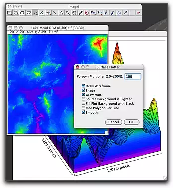
  The lake_mead_dem_8-bit_uncal.tif image is a Digital Elevation Model (DEM) of the Lake Mead area, where Nevada, California, and Arizona all come together. It's a good example of a synthetic image, since it was not taken with a camera of any type. Instead of brightness, each pixel value in the image represents (or is at least proportional to) the elevation at that location.
  
  
  Make sure the lake_mead_dem_8-bt_uncal.tif image is the active window by clicking on it. If you do not this, then you might be asking for a histogram on another window and end up with erroneous results.
• Choose Analyze > Histogram. A histogram window will open.
  Show me the histogram
  Hide
  

  
  
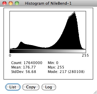
  The histogram shows a frequency distribution of pixel values in the image (or the selected part of an image). In other words, it tells you how many pixels (the Count) there are in the image for each different value from 0 to 255. Think of breaking all the little pixels apart and sorting them into piles with the same value, and arranging the piles in order, from lowest to highest value. Viewed from the side, the "mountain range" of pixel piles would look just like the histogram plot you see here.
  
• If you move your cursor across the histogram plot, the value (pixel value) and count (number of pixels in the image with that value) appear in the lower right corner of the histogram window. For example, we can confirm that there are exactly 3,862 pixels with a value of 118 in this image.
• If you want to see all of the counts for all of the pixel values, click the List button in the lower left corner of the Histogram window.
• Close the window containing the count table, but leave the Histogram and DEM windows open.
• A hot tip: If you select just a part of the image, the histogram will report statistics for only the pixels in the region (the Region Of Interest, or ROI) you selected!

Histograms are a basic tool for understanding the data in digital images. As you'll see in the next section, histograms can be a key to understanding digital images, deciphering any processing that has already been done to the image, and determining whether you can do any useful scientific analysis of the image.

Image Types

ImageJ refers to the bit depth and number of channels (such as color bands) of an image as its type. In this section, you will explore and learn some of the characteristics of the different image types available to you.

8-bit (grayscale, uncalibrated)

8-bit grayscale images are the most common type used with ImageJ, since 256 possible values is sufficient for most purposes, providing a good balance of image resolution and size.

• Still working with the Lake Mead DEM image, mouse around the image and look at the pixel values reported in the ImageJ status bar. Find the lake in the image. What pixel value in the image represents the elevation of the lake surface?
• Look at the histogram window. Can you see the surface of the lake in the histogram? How many pixels in the image represent the lake?
  Show me the answers
  Hide
  The lake surface is represented by the value 18. There are 64,900 pixels in the image with a value of 18.

  

  
  
• While you're here, try some of these other cool things you can do with DEM images to visualize the data in different ways;
• Apply different lookup tables to the image (Image > Lookup Tables).
Show me the result
Hide
This is how it looks with the 32_Colors lookup table.





• Threshold the image (highlight a range of pixel values in the image) by choosing Image > Adjust > Threshold. You can make the image look like the land is being flooded by water (or ketchup, since the default threshold color is red).
Show me the result
Hide

• Use thresholding to highlight only the elevation of the lake surface. (When you're finished, turn off thresholding by clicking the Reset button in the Threshold window.)
Show me the result
Hide

• Use Analyze > Surface Plot to re-create a 3-D view of the scene.
Show me the result
Hide

• Use one of the line selection tools to select a path through the scene, then create a profile plot along the path (Analyze > Plot Profile).
Show me the result
Hide

• Close all of the open image, histogram, and plot windows.

8-bit (grayscale, calibrated)

The pixel values in the previous image show relative elevation—pixels with higher values are higher in elevation than pixels with lower values. In a calibrated 8-bit image, the values provide actual elevation information.

• Download and open this version of the Lake Mead DEM image.
  lake_mead_dem_8-bit_calibrated (TIFF 1.4MB Jul16 11)
• Mouse around the image and look at the values reported in the status bar. What is different in this version?
  Show me the answer
  Hide
  There are two numbers reported, with one in parentheses.
  
  
  This image has been calibrated so that the pixel values from 0 to 255 are converted to elevation, in meters. The value in parentheses is the original 8-bit pixel value, and the number to the left of it is the calibrated elevation value. A calibrated image uses a formula to convert the "raw" uncalibrated pixel values to more meaningful, real-world measurements.
  
• Find the elevation of the lake surface in this image.
  Show me where to look
  Hide
  The elevation of the lake is about 325 meters above sea level.
  
  
• Create a histogram of this image. Notice that it now reports calibrated values. Again, can you see the lake surface in the histogram, both by the plot and by the modal (most frequently appearing) value in the image?
  Show me the histogram of the calibrated image
  Hide
  

  
  
• Close any open image and histogram windows.

If you ever need "quickie" images to practice with, demonstrate on, or just to amaze your friends, ImageJ has built-in links to more than 30 sample images of various bit depths, types, and subjects. Before moving on to the next image type, we will look at one of these sample images to review other basic principles of digital images.

• Choose File > Open Samples > Gel (105K).
  
  
  
  
• This is a scanned image of an electrophoretic gel (think "DNA fingerprint"). Look at the image window title bar. What type of image format is this?
  Show me the answer
  Hide
  This is a GIF (Graphic Interchange Format) image.
  
  
• According to the image window status bar, what are the dimensions, bit depth, and memory size of the image?
  Show me the answer
  Hide
  Width (columns) = 276, Height (rows) = 467, Bit Depth = 8, Memory = 126K.
  
  
• Mouse around the image. Where is the origin (0,0)? What are the coordinates of the pixel in the lower right corner of the image?
  Show me the answer
  Hide
  The origin of ALL images in ImageJ is the upper left corner. The coordinates of the lower-right pixel are (Width-1,Height-1). In this case, it's (275,466).
  
  
• Mouse around the image and look at the pixel values, shown in the ImageJ status bar. What is the possible range of pixel values in an 8-bit image? Choose Analyze > Histogram and find out the actual range (Min and Max) of the pixels in this image.
  Show me the answer
  Hide
  The range of possible pixel values in an 8-bit image are 0-255. In this image, the pixels range from 9 (darkest) to 200 (brightest).
  
  
• Does the memory size of this image makes sense? Each pixel in this image is represented by 8 bits, or 1 byte. The total number of bytes equals the total number of pixels. What is the total number of pixels (or bytes) in this image? How many kilobytes is this? (Reminder: When dealing with computers, the kilo- prefix means 2¹⁰ or 1024, not 1000. To convert from bytes to kilobytes, divide by 1024. To convert from kilobytes to megabytes, divide by 1024 again.)
  Show me the answer
  Hide
  Pixels = Width x Height = 276 x 467 = 128892 pixels. 1 kilobyte = 1024 bytes (1024 = 210) To get the number of kilobytes in the image, divide the number of bytes by 1024... 128892 / 1024 = 125.87 kilobytes (let's round it off to 126K!)
  
  
• When you opened the image, it said 105K (kilobytes)—not 126K. Why the difference?
  Show me the answer
  Hide
  Short Answer: The 105K is the amount of storage space the image FILE occupies on a storage device like a hard drive or memory stick. The 126K is the amount of your computer's memory (RAM) that the image occupies when it is open.
  
  Long Answer (Read at your own risk!): The gif image format is a compressed format. In other words, it mathematically stores the information in less space than the raw data—in this case, 105 kilobytes. The original data (or something close) is reconstructed when the image is opened, requiring 126 kilobytes of computer memory. The popular JPG format is another compressed format. When stored, the image file size is a function of many factors—the dimensions and bit depth of the image, the actual content of the image, the image format, and the type and level of compression used. When an image is opened in ImageJ (or any other computer application), the image size is determined ONLY by the width, height, and bit depth. That's why image files invariably seem to get "bigger" when you open them, and why a 249.7MB image may fail to open on your computer even though you have 300MB of memory available in ImageJ. No matter what format you use to store an image file, or how much room that file occupies on your hard drive, a 500 x 500 pixel, 8-bit image ALWAYS occupies 244KB of your computer's memory when it's open. Give it a try. Choose File > New > Image and create a new 500 x 500 pixel, 8-bit image filled with anything (or nothing). Look at the status bar of your new image—244K. No matter what the image is of, an image that size occupies 244K of memory. It's math, not magic, so it's predictable!
  
  

16-bit (grayscale)

• Close the Gel image and drag-and-drop this link to open a 16-bit version of the Lake Mead DEM into ImageJ.
  Lake Mead DEM (16-bit) (TIFF 2.8MB Jan27 10)
• This is the same image you worked with earlier, but in 16-bit format. Since 16 bits can represent values between 0 and 65536, this image can use the actual elevations (in meters) as the pixel values. Watch the value in the status bar as you mouse around the image.
• Now you can read out the elevation of the lake surface directly. What is it?
  Show me the answer
  Hide
  The elevation of the lake surface (the modal value of the image. is 329 meters above sea level.
  
  

  

  
  
  ImageJ can do all of the fun tricks (lookup tables, thresholding, surface and profile plotting, measuring, etc.) with 16-bit images that it can do with 8-bit images. (However, you're always limited to lookup tables with just 256 colors, which ImageJ spreads over the range of values in the image.)
  
  
  
• Spend a few minutes exploring this image, trying out the different visualization techniques you learned.
• When you are finished exploring the image, close all open windows.

The DEM was a synthetic image. Let's look at a 16-bit image created with a camera—this one attached to a telescope.

• Close the 16-bit DEM image and choose File > Open Samples > M51 Galaxy image.
This is an astronomical image of galaxy M-51. Since astronomical imaging involves a HUGE range of brightnesses, each pixel is represented by 16 bits or 2 bytes. That means that every pixel in the image can have any value between 0 and 65535. (20-1 and 216-1).


• Mouse around the image and look at the different pixel values. Note where the values are highest and lowest. Generate a histogram of the image to see the highest and lowest values in the image. What are they?
Show me the answer
Hide
The values in the M51 Galaxy image range from 0 to 10106.


• Calculate the memory size of this image based on its width, height, and bit depth. Does it match the reported size?
Show me the calculation
Hide
Memory size = 320px x 510px x 2bytes/px / 1024bytes/kilobyte = 318.75KB

ImageJ reports the size of the image as 319K, so these values agree. The value of 177K listed on the sample image submenu is the size of the image file stored on the server. The file size values are given here so you can estimate the time required to download the files.


One problem with images with bit depths greater than 8-bits per channel is displaying them. ImageJ (and most other computer applications and display systems) is limited to 256 different brightness levels in any one color channel. That means that the galaxy image is trying to display a possible range of 65536 brightnesses with only 256 shades of gray (or color). However, there is a way to better match the 256 available colors to the range of values in the image, or even to just a portion of that range to bring out detail in a small part of the image.


• Choose Image > Adjust > Window / Level to open the Window and Level control. Notice the little histogram at the top of the W&L window showing that most of the pixel values in the image are bunched together at the lower end. Click the Auto button to match the range of output (display) values to the input (image) values. Now M-51 looks more like a galaxy!
• You can even apply color lookup tables to bring out more of the fine detail or just to make it look cool. Try some different color lookup tables until you find one you really like. (Image > Lookup Tables)
• The color is not really a part of this image. When you apply a color lookup table to a grayscale image, the result is a pseudocolor image.
• Experiment with the Level and Window controls in the W&L window and note how they affect the image display. Just don't click the Apply button unless you want to permanently change the pixel values in the image.
• Close all of the open image windows.

32-bit grayscale

Another common scientific image data type represents measurements using 32 bits (4 x 8 bytes) per pixel. This type is often called "32-bit floating point" data, because the values are stored as positive or negative decimal values with a certain number of decimal places of precision. In effect, the pixel values are stored in scientific notation Thus, it you measure a temperature at some location as -17.6 degrees Celsius, you can code the pixel value as exactly -17.6 (-1.76 x 10¹. There's no need to density calibrate the image because the pixel values are the measurements. If necessary, scientists can increase both the range and precision of their measurements by using even more bits per pixel, such as 64-bit floating point data. ImageJ is limited to images with 32-bit floating point (also called "32-bit real" or "32-bit float") values.

A data source you are familiar with that provides images in 32-bit real format is the NASA Earth Observations (NEO) web site.

• Using your browser, go to NASA Earth Observations (NEO).
• On the NEO search page, click the Energy tab below the map display, and choose Solar Insolation, at the bottom of the Energy Datasets list. Take a minute to look at the most recent thumbnail image and the image scale. What units of measure do the pixels in this image represent? What are the minimum and maximum values that could be in the image?
  
  
  Show me the answer
  Hide
  The units of measure for Solar Insolation images are W/m2 (Watts per square meter). The scale ranges from 0 to 550 W/m2
  
  
• In the Search Parameters panel, select the Full Size, Color, GeoTIFF (floating point), and Solar Insolation (8 day) options, and click the Download button to download the TIFF file to your browser's default location.
  Be sure to choose the GeoTiff (floating point) and NOT the regular GeoTiff format.
  Show me the settings
  Hide
  

  
  
• Use ImageJ to open the image you downloaded.
• Mouse around the image and look at the pixel values. Notice that the pixel values reported in the ImageJ status bar are decimal values between 0 and 550, with no 8-bit values listed.
• To add a little color to this grayscale image, choose Image > Lookup Tables > and choose one of the built-in color tables. Don't worry that you can't find one to match the original color scale exactly.
• Choose Analyze > Show Histogram. Notice that, like 16-bit images, the Histogram command opens a dialog box that lets you specify histogram options. Click OK to use the default values.
  Show me the histogram
  Hide
  

  
  

• Close any open image windows.
• Use the NEO web site to download a 32-bit grayscale NDVI (Normalized Differential Vegetation Index) image, at the bottom of the LIFE tab. If you can't download and open an image for some reason, you can use the one here.
32-bit NDVI TIFF (TIFF 24.7MB Jul16 11)
• Look at the legend below the image on the NEO web page. What are the minimum and maximum values for an NDVI image? What is the middle value? (Remember or write them down. They will come in handy soon.)
  Show me the NEO page
  Hide
  

  
  
• Open the image in ImageJ. How does the image look when it first opens?
  Show me the answer
  Hide
  When the 32-bit NDVI image opens, land areas look black and oceans are white.
  
  

  

  
  
• Mouse around the image. Does the land really all have the same value?
  Show me the answer
  Hide
  No, the land areas have pixel values between -0.1 and 0.9.
  
  
• What is the value of the pixels that represent the ocean? Why?
  Show me the answer
  Hide
  Ocean pixels are assigned values of 99999.0. This is a "no data" value, because NDVI is only relevant to land areas.
  
  
• Make a histogram for this image. Use 256 bins, set the X Min to the minimum value you recorded from the legend and the X Max value to the maximum value from the legend, and click OK.
  Show me the resulting histogram
  Hide
  

  
  

  

  
  
• Can you explain why the data is there, but you can't see it?
  Show me the answer
  Hide
  The no data value (99999) is incorrectly read by ImageJ as the maximum data value, so it has binned the grayscale lookup table to cover the full range of values from -0.1 to 99999. All of the actual data are binned to the values near the lower (black) end of the lookup table.
  
  
• Use the Window and Level control to make the lookup table better fit the range of the actual data. Click the Set button in the W&L window, enter 0.4 as the center value and 1 as the Window Width, and click OK. Do you see why you used those values?
  Show me an example
  Hide
  The data values range from -0.1 to 0.9, a range (width) of 1. The center of that range is at 0.4 (remember the legend?)
  
  

  

  
  
• Add an attractive color lookup table to the image to make it a pseudocolor image.
  Show me an example of a pseudocolor NDVI image
  Hide
  

  
  
• Mouse around the NDVI image for a few minutes and be sure you understand what it's showing you. (In a nutshell, low values show where vegetation is absent or unhealthy and higher values indicate vegetation with more "vigor".)
• Close the NDVI image.

24-bit RGB (True Color)

You have displayed some grayscale images as pseudocolor images by applying color lookup tables. How are realistic, true color images created?

• Choose File > Open Samples > Nile Bend (1.9M). This is a satellite image showing the Nile River in Egypt.
• Look at the image window title bar. What type of image format is this?
Show me the answer
Hide
This is a 24-bit RGB .jpg (JPEG) image.


• According to the image window status bar, what are the dimensions, bit depth, and memory size of the image?
Show me the answer
Hide
Width (columns) = 4200, Height (rows) = 4200, Bit Depth (RGB) = 24-bit (8+8+8 bits), Memory = 67MB.


• This image was saved in RGB format, so each pixel is represented by three bytes—a red value, a green value, and a blue value. Mouse around the image and zoom in, if you want. Position your cursor over one of the pixels that represents vegetation near the river. What do you notice about the R, G, and B values that confirm that the pixel you chose is green?
Show me the answer
Hide
The green (G) value is greater than the R (Red) and B (Blue) values.


• Calculate the memory size of this image. There's a catch though. In ImageJ, all RGB images actually use 4 bytes for each pixel. One byte represents red, one green, one blue, and the fourth is called an alpha channel. This one is used to hold other information you don't see. This image type is also referred to as RGBA.
Show me the calculation
Hide
Image size = 4200px x 4200px x 4bytes/px / 1024 bytes/kilobyte / 1024 kilobytes/megabyte = 67.29MB, which rounds to 67MB.


RGB images don't need a color lookup table to display the image. A fundamental characteristic of 24-bit color images is that the appearance of each pixel is defined by three separate 8-bit values, each representing the brightness at that location in one of the three light primary colors—red, green, and blue. Think of the pixel's RGB values as its color "recipe". For example, if you mix together 67 units of red, 23 units of green, and 51 units of blue, the pixel would be a dark magenta color.


• Make a histogram of the 24-bit RGB NileBend image, and keep it open.
Show me the RGB histogram
Hide



• Don't try to interpret the histogram just yet. It should make sense to you in a few minutes.
• Keep the NileBend image window open.

8-bit Color (Indexed Color)

You may also work with color images in 8-bit color format.

• ImageJ can convert between different image formats, when necessary. You are going to convert this 24-bit color image to 8-bit color. Before you do, predict the new image's memory size. (RGB = 4 bytes per pixel; 8-bit = 1 byte per pixel)
Show me a hint
Hide
Since the number of bytes for each pixel is reduced from 4 to 1, the grayscale image should require 1/4 as much memory. 67.29MB / 4 = 16.8MB, which rounds to 17MB.



Indexed Color

RGB values can represent over 16 million different colors. By converting to 8-bit color, that palette is reduced to just 256 colors (two of which are black and white). During the conversion, ImageJ does some fancy math based on statistics and the science of color perception to determine the 256 most important colors for this particular image, then creates a unique color lookup table containing just those colors. The palette for this image will have mostly shades of grays, tans, and dark greens. A different scene would have a lookup table with a different palette of colors. ImageJ assigns a new numerical value to each pixel based on the index—the number that corresponds to each position in the lookup table—of the color closest to that of the original pixel.


• Choose Image > Type > 8-bit Color, select 256 colors, and click OK to convert the image. Watch carefully—do you notice much change in the appearance of the image?
• Mouse around the image and look at the values in the ImageJ status bar. Notice how they are different from what was reported for the RGB version. A new value, the Index is reported. This is the position of that color on the new lookup table, and the Value to the right of the index is the RGB "formula" for that color. This image has been literally reduced to a "paint by numbers" picture!
  Show me the status bar
  Hide
  

  
  
  What is the reported memory size of the image? How does it compare to your prediction?
  
  
  Show me the answer
  Hide
  The reported memory size is 17MB, which should match your prediction.
  
  
• Create a histogram for the 8-bit color image and leave it open.
  Show me the 8-bit Color histogram
  Hide
  

  
  
  This histogram shows the new color lookup table as a horizontal bar just below the histogram graph. The histogram graph itself now appears as a random pattern of vertical lines, nothing like the RGB histogram. Keep this histogram window open for comparison.
  

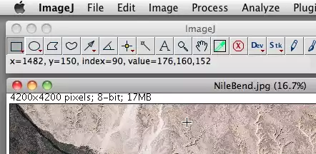
Converting Between Image Types

ImageJ can convert back and forth between most image types. This is a useful feature, but let's see if there are any down sides to image type conversion.

• Choose Image > Type > RGB Color to convert the 8-bit color image back to 24-bit RGB.
• Create another histogram of the RGB Color image and compare it to the original histogram.
  Show me the RGB histogram
  Hide
  

  
  

What happens to the image data when you convert from a higher bit depth to a lower bit depth? (Example: From 16-bit to 8-bit)

Show me the answer

Hide

How about converting the 8-bit color image to 8-bit grayscale—where would that get you?

• Choose Image > Type > 8-bit.
• Create a new histogram and leave it open.
Show me the histogram for 8-bit color converted to 8-bit grayscale
Hide



Explain what this histogram shows.


Show me the answer
Hide
This histogram shows the overall shape of the original RGB image histogram, but the gaps tell you there are fewer unique values in the image. In other words, detail in the depth dimension has been lost.


What happens to image data when you convert from a lower bit depth to a higher bit depth? (Example: From 8-bit to 16-bit) In other words, can you gain back lost pixel data by simply converting back to the original bit depth or by further changing the data type?


Show me the answer
Hide
Reducing ANY dimension of an image (width, height, or bit depth) destroys data and changes the remaining pixel values. Scaling up to the original dimensions does NOT restore any missing data, and may create false data.


So, when you have scaled an image or changed it to a different type, how can you get back to the original data?


Show me how
Hide
To get back to your original image data, either;


• Choose File > Revert.
• If Revert does not work, you must close the image (without saving it) and re-open or import it.
• Choose File >Revert to revert to the original RGB color image. Leave all of the histogram windows open. If you recall, the first histogram you created of the Nile image was for a 24-bit RGB version. It's time to come full circle and return to that histogram.
  
• Choose Image > Type > 8-bit to convert the RGB color image to 8-bit (grayscale).
• Make a new histogram of the 8-bit grayscale Nile image and compare it to the original RGB color histogram you made. What do you notice? What does that tell you about 24-bit color image histograms?
  Show me the original RGB histogram and the 8-bit grayscale histogram
  Hide
  Here's the original RGB Color histogram:
  
  

  

  
  
  And here's the histogram of the 8-bit grayscale version of that image:
  
  

  

  
  

They are exactly the same! When you create a histogram from a color image, the values are first converted to grayscale equivalent values. By the way, ImageJ does not convert R, G, and B values to grayscale by simply averaging them. The conversion equation weights each color channel to match how each color contributes to your perception of brightness. The formula it uses is: 30% Red + 59% Green + 11% Blue. You could confirm this by choosing a pixel in the original RGB image, write down its RGB values, run them through this formula, then look up the value of the same pixel in the 8-bit grayscale conversion of the same image.

File Formats for Science

In everyday life, users are interested in the appearance of images and videos and having a simple, inexpensive, yet pleasing user experience—pictures are sharp and colorful and video playback is smooth, with good sound. Consumer-oriented file formats provide these qualities while allowing the files to be sent quickly over computer and phone networks and maximizing the number of pictures and videos that can be stored on a device.

Scientists have a different set of priorities. Their images, both still and "moving", contain important information that often needs to be preserved in a form that retains all of the original data. Scientists often use consumer file formats like JPG, GIF, BMP or movie files such as AVI, MOV, WMV, and FLV, but sometimes they need to preserve the original measurement values for each pixel in their images. This is where file formats like TIFF (Tagged Image File Format) and (Flexible Image Transport System) come in, because they are better suited to storing the metadata that are important for scientific tasks.

FITS is used mainly by the Astronomy community. FITS is much more than an image format (such as JPG or GIF) and is primarily designed to store scientific data sets consisting of multi-dimensional arrays (1-D spectra, 2-D images or 3-D data cubes) and 2-dimensional tables containing rows and columns of data. Unlike other file formats, both FITS and TIFF files can contain one or many related images plus their metadata. ImageJ Is able to open most TIFF and FITS files, and can save single images in both formats.

ImageJ can open and save images in many different file formats. Some formats you're familiar with, and some you've never heard of and may never use. Without going into great detail, it's useful to be familiar with a few of the more common image file formats, and their pros and cons. In other words, "Why would I want to use this format instead of that format?"

TIFF (Tagged Image File Format)

• Data Types – Almost unlimited. Virtually any size, bit depth, number of channels, and number of layers (slices)
• Pros – Lossless—no loss of information due to compression. The gold standard image format for scientific imaging. Can store multiple images (stacks) and multiple channels (bands) in one file. Can store all calibration data, including location data (GeoTIFF).
• Cons –Image files are generally large, though ImageJ can directly open zip-compressed TIFF files without unzipping (try it!). TIFF files do not display consistently on web pages and take longer to transfer over networks.
• Uses and Recommendations –TIFF is ImageJ's native file format. It is recommended for general-purpose scientific imaging. It is the only common format that saves spatial and density calibration, overlay layers, and geographic information. It is also the only format that directly supports multi-dimensional stacks in ImageJ, including all calibration information.

JPEG (Joint Photography Experts Group)

• Data Types – Single 8-bit grayscale and 24-bit color images only. (no stacks)
• Pros – With moderate to high compression settings, files can be very small. Can be opened by nearly all imaging software and used in print and web publication. Plays nicely on the web.
• Cons –"Lossy" compression sacrifices pixel values for small file size.High compression settings produce artifacts that are easily seen in magnified images. Images lose their spatial and density calibration information. Limited choice of data types.
• Uses and Recommendations – Okay for spatial measurements where you only need to detect the locations of features, but avoid JPEG if you are making any type of density (pixel value) measurements.

GIF (Graphic Interchange Format)

• Data Types – Uses an indexed lookup table, so bit depths vary from 1 to 8 bits. Converted to 8-bit indexed color when opened. Stacks can be saved as Animated GIF format, but results are not always predictable.
• Pros – For the right types of images (graphic, not photographic), files can be very small. Can be opened by nearly all imaging software and used in print and web publication.
• Cons – GIF does not save spatial or density calibration information. Very limited choice of data types.
• Uses and Recommendations – Used mainly for graphic images (charts, graphs, etc.) with a limited number of colors. Generally used by graphic images downloaded from web sites, including thematic maps with large areas of the same color.

PNG (Portable Network Graphics)

• Data Types – 8-bit, 24-bit RGB, and 32-bit RGBA, both still and video (in uncompressed AVI format).
• Pros – Lossless—no loss of information due to compression. For the right types of images, files can be very small. Can be opened by most imaging software and used in print and web publication.
• Cons – PNG does not save spatial or density calibration information. Less compression for photographic images.
• Uses and Recommendations – PNG was developed as a replacement for GIF for web-based images and graphics. It provides good compression for some types of images, but does allow the user to select the level of compression. PNG is lossless, so the data (pixel) values are preserved.

To repeat a VERY important point—no matter what file format is used to store an image or how small that file is, the amount of computer memory the image occupies when the image is open is determined only by the dimensions of the image—its width, height, and bit depth. In image processing, then, other than conserving storage space, there's no advantage to saving images in JPG format, and there may be some serious disadvantages. We're not suggesting that you never use JPEG format, but it's a good idea to be aware of what happens when you do use it for your images. JPEG compression (quality) settings in ImageJ range from 0 (high compression, low quality) to 100 (low compression, high quality).

Your Assignment: Locate a Digital Image, Analyze It, and Describe Its Characteristics in Detail in Terms of Bit Depth and Pixel Histogram Distribution

1. Spend several minutes opening and exploring the other sample images. Several of the samples are multi-image stacks. You can look at the stacks now, but don't spend too much time analyzing them—you will look at them in more detail in Part 2. For the single images, examine all of the basic aspects of the image: dimensions, data type, histogram, etc. You are using ImageJ primarily to view and analyze earth science data, but you can tell from these images that it is a general-purpose tool that can be used with any type of digital image.
2. Choose one of the sample images or ANY other digital image you like, create a histogram of the image, and create a screen capture showing the image and its histogram.
3. Go to the Part 1: Share and Discuss Page, post the screen capture and describe as much as you can about it, in terms of the characteristics explained in this section (e.g. bit depth, histogram data).

Screenshot Instructions for Mac Users

• Press Command-Shift-4 (Command key = Apple key) all at the same time and drag a box over the area of the screen that you want to capture. Depending upon your operating system, this will produce a file named Picture1.png or Screen shot Date Time.png on your desktop. Move the screenshot to your Day 1 folder or to a place where you can easily find it. Double click on the file to open it in Preview. Rename the image and save it as a jpeg, giving it a name that describes it, such as Lake_Mead_pixel_zoom.jpg.

Screenshot Instructions for PC Users

• Press Alt and Printscreen at the same time. This will save an image of the screen to the computer's clipboard.
• Launch Paint and choose Edit > Paste.
• Save the image as a jpeg, giving it a name that describes it, such as Lake_Mead_pixel_zoom.jpg.

Resources

• The ImageJ User Guide provides additional information about bit depth and image file formats.

Source