
Flood Frequency and Urbanization
Aberjona River Watershed, Massachusetts
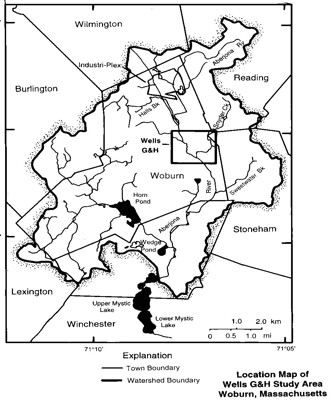 Location of the U.S. Geological Survey gage on the Aberjona River in Winchester, Massachusetts relative to the location of the Wells G & H Superfund Site in Woburn (modified from Joseph, 1995).
Introduction
Surface water and groundwater flow systems are often highly interconnected and interdependent. Flooding can be the result of several interrelated variables including the connection between surface water and groundwater. This exercise uses analytical tools employed by water scientists to understand the probability of flooding within a watershed and how flood frequency can be impacted by changes in land use.
We begin by examining the historic character of the Aberjona River to help forecast future behavior of the flow system. The gaging station at Winchester, Massachusetts at the southern end of the Aberjona River watershed (see figure) is used to depict historic streamflow records.
Part I Flood Recurrence Intervals
The flood recurrence interval (return period) for a stream is the probability that a flood of a given magnitude will be equaled or exceeded in a given year. A flood having a recurrence interval of 10 years has a 10% chance of recurring in any year; a 100-year flood has a 1% chance of recurring each year. To compute recurrence intervals, annual peak streamflow values (i.e., annual peak discharge values) at a stream gage are needed. In this assignment, we use data collected for the U.S. Geological Survey national stream gaging network (water.usgs.gov/nwis/) at the Winchester, Massachusetts gaging station (USGS Gaging Station 1102500). Streamflow data have been collected at this location since 1939. The annual peak daily discharge has been identified for each water year (Oct. 1 to Sept. 30) from 1940 to 2001 (62 years of record) and appears in the "Aberjona Peak" worksheet. This table shows the gage height and the peak discharge value for each water year. Using the instructions below, assign rank values to the peak flows and then compute recurrence interval for each annual peak discharge. See Reference Book for more information.
Instructions
- Sort the annual peak discharge data from largest to smallest (descending order), according to the peak discharge (see EXCEL TIPS), and assign a rank in the appropriate column in the "Aberjona Peak" worksheet (largest annual peak discharge = rank of 1). Calculate the river elevation using a gage elevation of sea level (zero). Note no gage height was measured for the March 22, 2001 peak flow.
- Calculate the recurrence interval of each annual peak discharge using the flood frequency equation 4-4 in the Reference Book.
- Plot the annual peak discharge values versus the recurrence interval values with recurrence interval on the X-axis and peak discharge on the Y-axis. See EXCEL TIPS in Reference Book for plotting help.
- Select (XY) scatter plot.
- Highlight the recurrence interval values and annual peak discharge values (The peak discharge data are repeated on the right side of the data table to make plotting easier.)
- Chart title should be "Part I - Aberjona River 1940-2001"
- X-axis label should be "Recurrence Interval (years)"
- Y-axis label should be "Discharge (cfs)"
- Y-axis scale minumum is 0 and maximum is 1800
- Convert the X-axis to a logarithmic scale. The relation between recurrence interval and annual peak discharge should become more "linear" when it is plotted on a semi-logarithmic scale graph.
- Use EXCEL to calculate the equation of a trend line through the data. This will be a logarithmic relation because it is a semi-logarithmic plot. This equation will serve as your model for forecasting future flood characteristics. Add gridlines to both the X and Y axes (see EXCEL TIPS in the Reference Book).
- Answer the Part I questions on the "Questions" worksheet using a print out of the flood frequency graph and data analysis. (The graph should have the appropriate labels with units indicated.)
Part II Land Use Impacts
Land use within the Aberjona River watershed has changed markedly over the past 60 years. The region has gone through an evolution from farms and greenhouses to an industrial base of warehouses, strip malls, office buildings, and parking lots. See the Reference Book and problem setup materials for photographs and a more in-depth discussion of land use changes in the watershed.
The following figures show the average deviation of recharge (precipitation) from average values and annual peak flow discharges plotted against time. Notice that the annual peak flow data appear to show an increased variation in peak flow after approximately 1955. Some questions that one might ask include: What is the cause of this apparent trend? Also notice that the amount of impervious land surface (paved areas, buildings, etc.) increased from less than 5% pre-1956 to greater than 35% post-1978. Is there a relation between these two factors? As more impervious surfaces are created, do you observe more "flashy" behavior in the stream and thus higher annual peak discharges? The second part of this exercise investigates this apparent relation between land-use practices during this time period and stream discharge behavior.
If the stream flow characteristics changed due to land use practices, then flood frequency probabilities would also have to change to reflect the higher runoff rates following creation of all the impervious surfaces. Test this hypothesis by examining two portions of the annual peak discharge record (one pre-1956 and one post-1978).
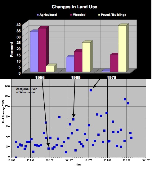 Annual peak flows for the Aberjona River at Winchester, Massachusetts along with land-use changes from 1956, 1969, and 1978 (Metheny and Bair, 2001).
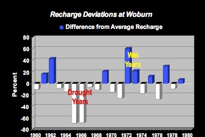 Recharge (precipitation) deviation from the average annual precipitation from 1960 to 1981 in Woburn, Massachusetts (Metheny and Bair, 2001).
Instructions
- Worksheet "Pre-1956" contains annual peak discharges for water years from 1939 to 1956. Worksheet "Post-1978" contains annual peak discharge data for water years 1978 to 1994. Sort the annual peak discharge data from largest to smallest (descending order), according to the peak discharge (see EXCEL TIPS) and assign a rank in the appropriate column, as you did in Part I of this exercise.
- Calculate the recurrence interval of each annual peak discharge using the flood frequency equation 4-4 in the Reference Book.
- Plot the annual peak discharge values versus the recurrence interval values with recurrence interval on the X-axis and peak discharge on the Y-axis. See EXCEL TIPS in Reference Book for plotting help.
- Select (XY) scatter plot.
- Highlight the recurrence interval values and annual peak discharge values. (The peak discharge data are repeated on the right side of the data table to make plotting easier.)
- Chart title should be "Part II - Aberjona River Pre-1956" or "Part II - Aberjona River Post 1978"
- X-axis label should be "Recurrence Interval (years)"
- Y-axis label should be "Discharge (cfs)"
- Y-axis scale minumum is 0 and maximum is 1400
- Convert the X-axis to a logarithmic scale. The relation between recurrence interval and annual peak discharge should become more "linear" when it is plotted on a semi-logarithmic scale graph.
- Use EXCEL to calculate the equations of a trend line through the data. This will be a logarithmic relation. As before, this will serve as your model for forecasting future flood characteristics. Add gridlines to both the X and Y axes (see Reference Book).
- Answer the Part II questions in the "Questions" worksheet using a print out of the two flood frequency graphs and their data analysis. If additional calculations and graphs are used to answer the questions in Part II then print out these materials used to support your answers.
Materials
- Flood Frequency Data (Excel 63kB Jul6 06)
- Flood Frequency Questions (Microsoft Word 30kB Jul11 06)
References
Joseph, J.A., 1995, A Hydro-Geochemical Assessment of Groundwater Flow and Arsenic Contamination in the Aberjona River Sub-basin, M.S. thesis, Department of Civil and Environmental Engineering, MIT.
Metheny, M. and E.S. Bair, 2001, The science behind "A Civil Action"; hydrogeology of the Aberjona River, wetland, and Woburn wells G and H, in Guidebook for geological field trips in New England. Geological Society of America, p. D1-D25.
Rutledge, A.T., 1998, Computer programs for describing the recession of ground-water discharge and for estimating mean ground-water recharge and discharge from streamflow data—update: U.S. Geological Survey Water-Resources Investigations Report 98-4148, 43p. http://water.usgs.gov/pubs/wri/wri984148/