Forecasting River Discharge and Runoff with a Python-based Statistical Machine Learning Tool
Introduction
In the face of an uncertain climate and increasing extreme weather events, it is challenging to predict river discharge and surface runoff. Efficient forecasting helps all aspects of watershed management, including drought resilience, flood preparedness, water availability for irrigation in croplands, among others. Machine Learning can efficiently forecast river discharge or runoff based on past data, but understanding the basic concept of Machine Learning, let alone developing a Machine Learning tool, can be difficult. Furthermore, an easy-to-use yet efficient Machine Learning tool that can forecast river water conditions is not always readily available. Here we introduce an online Python tool based on ARIMA (Autoregressive Integrated Moving Average) to predict streamflow or runoff events for any location around the world.
This tutorial will demonstrate how to automatically and instantly download river discharge for any user-defined duration and location within the United States, and surface runoff data around the world, and integrate the data in ARIMA to produce future forecasts for any defined period of time.
To run the default version of the tool, you will be accessing river discharge data from the US Geological Survey - Current Water Data for the Nation (USGS) or from NASA's Global Land Data Assimilation System (GLDAS-2). In this tutorial, we will use two locations as an example for either dataset: Jacksonville, Florida for the USGS dataset, and Istanbul, Turkey for the GLDAS-2 dataset.
The tool has two unique features:
(1) It is an end-to-end workflow that performs all data discovery, download, pre-processing, and analysis tasks in a semi-automatic manner.
(2) Users can run this tool simply in a web browser without having to write python code or installing any software in personal computers.
Tool URL: https://colab.research.google.com/drive/1Tiq1I80VIpKOHQOtek7aHKSMJqswhcU9
Video Demonstration: https://youtu.be/jUXCHcxw-Ig
Conceptual Outcomes
- Users will understand how to utilize and implement Machine Learning for forecasting river discharge or runoff, and therefore gain an awareness of future environmental conditions.
- The data derived from this tool will equip users with the essential insights into effective prediction of drought, flood, and water availability in general for any defined location for any specified period of time.
Practical Outcomes
- By completing this tutorial, users will learn how to develop and run python codes easily using a web-based platform called Google Colaboratory.
- Users will get hands-on training on end-to-end discovery, integration, and analysis of complex streamflow or runoff data.
- Users will learn how to instantly forecast river discharge or runoff using ARIMA.
Time Required
It would take roughly 45 minutes to complete this tutorial. The required time may vary depending on the selected location and the internet connection quality.
Instructions
Read this short tutorial carefully to set up your Google Colaboratory:
Let's start by clicking on the link below: (This will open a Python code in your computer's browser).
https://colab.research.google.com/drive/1Tiq1I80VIpKOHQOtek7aHKSMJqswhcU9
Watch this instructional video to make yourself familiar with all the steps followed in this tutorial. You will see how we extracted river discharge or runoff data and applied a statistical machine learning tool to generate future forecasts for our desired location of interest.
Execute every step by merely clicking the play button or pressing "Ctrl+Enter." You can run the tool for any area of interest both in the United States and worldwide.
Relevant notes associated with each step are provided below.
If this is the first time you have used this tool, please begin by saving a copy of the tool in your Google Drive.
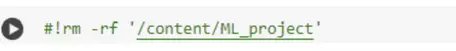
If this is NOT the first time you have used this tool, please edit the following line of the code in your previous copy by deleting the "#" symbol, then press the play button. Pressing the play button will clear any data that you have generated by this tool in your previous attempts.
![[creative commons]](/images/creativecommons_16.png)
Within each step are several cells to run. Be sure to run every cell within each step to avoid receiving any errors. If a step is skipped and an error occurs, go back to this cell, delete the "#"symbol and press play. Then proceed to Step 1 and start from the beginning.
STEP 1:INSTALL PYTHON MODULES
Run the cell by pressing the "play" button.
STEP 2: IMPORT PYTHON MODULES
In this step, you are going to "call" the python packages/modules that you installed in the previous step.
Once you call them, those packages/modules will be ready to perform specific geospatial functions in the subsequent steps.
STEP 3: LINK YOUR TOOL WITH GOOGLE EARTH ENGINE
For this step, users will need to set up a Google Earth Engine account using their own gmail ID. See this guide for more information.
After creating your Google Earth Engine account, replace the following line of code with your project ID (where the code reads "h2i-lab" is where you will replace with your ID in quotations).
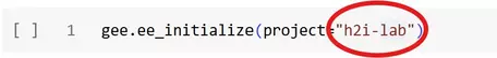
Edit the above line of code where it is indicated with quotations and replace it with your project ID.
After replacing the section of code with your project ID, you may run the code. Google will prompt you with a request for access to your Google Earth Engine account. Press "Allow," then select your account you used to set up Google Earth Engine.
Note: if this is NOT your first time running this tool, you will need to create a new project ID in Google Earth Engine, or else you will receive an "error" message.
STEP 4: DEFINE FUNCTIONS
Run the line of code to define the parameters in which the model will operate.
STEP 5: SELECT YOUR DESIRED DATASETS
In this step, you will select your dataset of choice. Selection of your dataset will give the tool direct access to river discharge or runoff data for your desired location. (Note that river discharge is also known as streamflow).
IMPORTANT: Your selection of which dataset is dependent on where you have selected to study.
The tool provides TWO options:
OPTION ONE: The USGS Streamflow Data: Selecting this dataset will limit the tool to river discharge data from a platform called USGS Current Water Data of the Nation, which provides data only in the United States1.
To access the USGS dataset, first:
- Run the code and enter "1" in the textbox.
- Provide the USGS monitoring station number of your choice. You must know your desired USGS monitoring station number and the duration of data available at that station prior to running this tool. You can find this information by browsing the interactive map on this website: https://waterdata.usgs.gov/nwis/rt.
- Specify the start and end dates of the dataset.
This will tell the model which location and USGS station to pull data from, and from which period of time it should base predictions on.
In this tutorial we are using a monitoring site in Jacksonville, Florida, and the date range from 2010 to 2017. After you have entered the correct station number, prompt the next step by pressing the "enter" key.
USGS Monitoring Station Number: 02246500
From Date: 2010-04-22
To Date: 2017-04-22
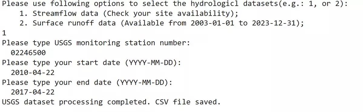
IMPORTANT: users must input their data range exactly in the format shown above (YYYY-MM-DD). However, the monitoring station and date range displayed in this tutorial are purely for demonstration purposes. This tool is available for analysis of any desired location and date range.
- Side note: You may encounter an error message if your selected start or end date does not align with the data available for your chosen station. For example, if you select 2010-01-01 as the start date for a USGS station, but data for that station begins on 2010-03-01, an error will occur.
OPTION TWO: The NASA GLDAS-2 ~25-km Surface Runoff Data: covers runoff data worldwide from 2003-20232. GLDAS-2 gets periodically updated to include data from recent years. Select this dataset if your desired location is outside the United States. To access GLDAS-2, follow these steps:
- Run the code and input "2" in the textbox.
- Specify the beginning and end dates of study (DD-MM-YYYY)
- Browse over the map and zoom in on your location of interest.
- Next, click on "Draw a circle maker" on the left panel of the map.
- Move your cursor to the desired location and left-click on the map.
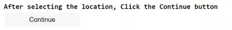
- Finally, after selecting your location, click "continue" at the bottom of the map.
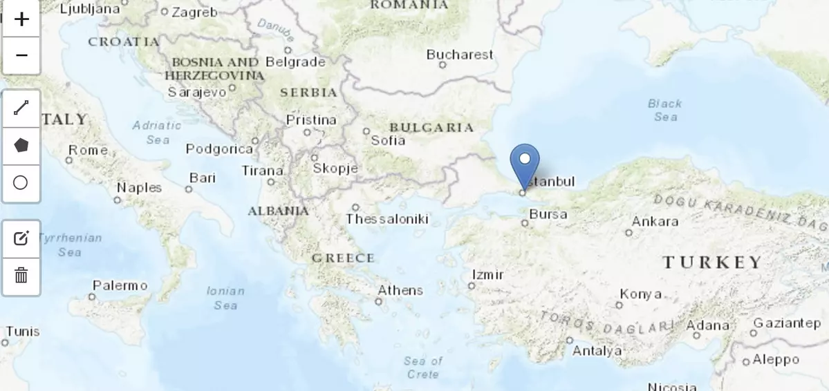
For this tutorial, we are using Istanbul, Turkey as our location of choice. After selecting your location, be certain to hit "continue" at the bottom of the cell. Wait until you see "GLDAS processing completed and CSV file saved" before moving on.
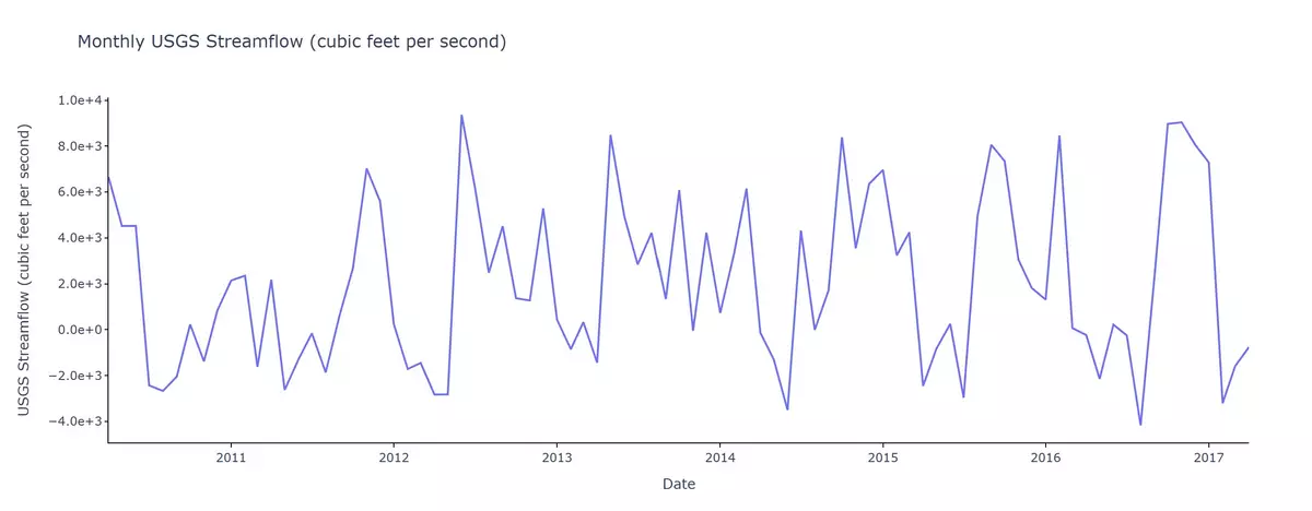
STEP 6: GENERATE A TIME SERIES PLOT USING YOUR SELECTED DATASET
This step will instantly generate a monthly streamflow in cfs units (cubic feet per second), or surface runoff in mm units (depth of water in millimeters).
Streamflow & surface runoff correlate to the amount of water in a watershed3; thus, by using a time-series plot to analyze streamflow/runoff data, we can gauge water levels over time and draw conclusions about weather conditions (e.g. frequency of storms, severity of events, compound variables, trends, etc.). This process allows us to make weather predictions with only past observations.
Time-series plots are commonly used for analysis of climate and hydrology data. Note that the following plots below display only past data, not future predictions.
The following is a time-series of streamflow for Jacksonville, Florida. The data used to generate the plotted time-series is issued directly from the USGS monitoring site. The observed peaks indicate periods of higher discharge which usually follow storm events.
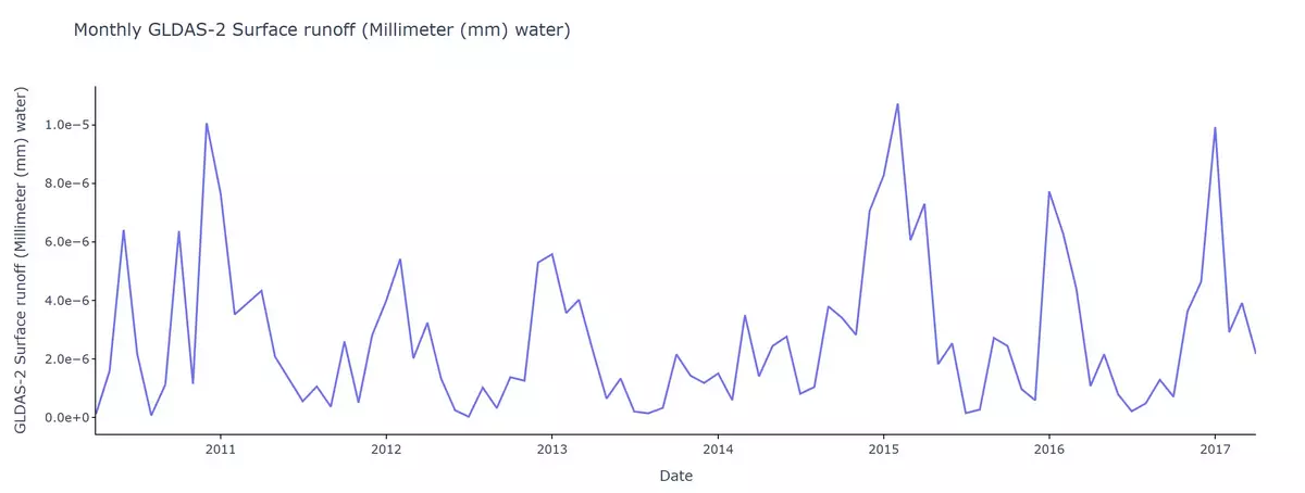
Below is a time-series of runoff for Istanbul, Turkey, measured in millimeters (mm). Similarly, the data used to generate the plot was issued directly from the NASA GLDAS-2 dataset. Just like in the streamflow time-series, peaks in runoff time-series correspond to storm events. Consider the valleys, or the low runoff values, in the time series. Can you think about what these might correspond to in real-world conditions?
STEP 7: RUN THE MACHINE LEARNING TOOL TO PREDICT FUTURE STREAMFLOW/RUNOFF DATA
This step will assess the data previously accessed in Step 5 to generate future streamflow and runoff data using ARIMA (short for "Autoregressive Integrated Moving Average"). These models are most often used to forecast future values based on historical data,4 essentially predicting how a variable will behave over time by analyzing patterns in past observations. It is best-suited for datasets that are recorded over regular intervals like daily, weekly, or monthly periods, like the streamflow or runoff data used in this tutorial. Besides climate and hydrology, ARIMA is widely used in fields like economics and business to forecast sales, stock prices, and other time-dependent variables.5
It will take ARIMA some time to complete its evaluation of the data we've inputted. Allow this cell to run completely before moving onto the next step.

STEP 8: GENERATE THE STREAMFLOW/RUNOFF PREDICTION
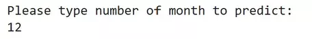
This step will prompt a response from the user to enter the number of months in which you would like the machine to predict streamflow and surface runoff for the desired location of study. In this tutorial we have chosen to predict 12 months ahead of our indicated end date of April 4th, 2017. Of course, you can choose any amount of time for your prediction.
Type out your selected number of months in the textbox prompt as seen below, then hit 'Enter.'
Proceed to call the next cell before moving onto step 9.
STEP 9: PLOT MACHINE LEARNING AND PAST DATA IN ONE FIGURE
In this step, you will generate a new time-series plot that displays both past data and the Machine Learning prediction. For our tutorial, we have used ARIMA to produce streamflow and runoff forecasts for 12 months ahead of time.
Note: The accuracy of ARIMA forecasts depends on the amount of past data available and the length of the prediction horizon. Shorter datasets and longer forecast periods (e.g., 18 months, 24 months, etc.) can lead to less accurate predictions.
The following is the streamflow time-series plot of Jacksonville, Florida generated in Step 6, overlaid with the machine learning prediction from step 8.
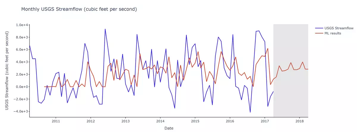
Observe the peaks. The red line represents the predicted dataset created by the model using machine learning. The blue line represents the past streamflow data derived from the USGS monitoring station in our location of choice (Jacksonville, FL).
Note the section in gray. The peaks in red depict what the model predicted for the 12 months following the end date of the input past data (blue line).
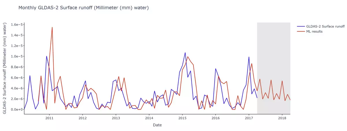
Now, let us look at the time-series plot generated for Istanbul, Turkey. Similarly, this is a plot that displays both the past runoff data accessed from GLDAS (seen in blue) and the machine learning tool's prediction (seen in red).
The section in gray represents the 12-month period that the tool had forecast based on the inputted data.
Can you see how simple statistical Machine Learning can be valuable in providing insight into future probable conditions?
STEP 10: EVALUATE THE ACCURACY OF THE PREDICTION
This step will evaluate the accuracy of the Machine Learning prediction by comparing the generated results with past data. To assess the model accuracy, this tool generates a chart with statistical values for both the input past data and machine learning data. Before we evaluate both, let us define a few statistical terms.
Count in statistics refers to the number of occurrences or observations of data points. Mean is the average value of the entire dataset. Standard Deviation (STD) is a measure of the amount the values in a dataset vary from its mean. Minimum/Maximum values represent the highest peak and lowest valley observed in a dataset.6
The statistics below were generated from the streamflow plots for Jacksonville, Florida at ft3/sec. Note that the columns at the top are labeled for the user to distinguish which values were generated by Machine Learning and which were derived from past data.
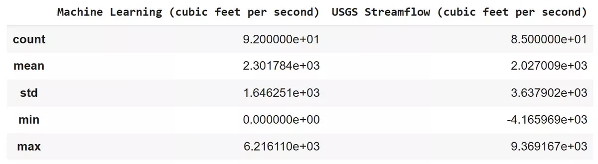
Proper interpretation of these values can tell us how effective ARIMA is at predicting future streamflow or runoff data in their location of choice.
In the case of Jacksonville, FL, the model predicted a slightly higher mean (2301.78 ft3/sec) than was observed (2027.01 ft3/sec), a higher minimum (0.0 ft3/sec), and a lower maximum (6216.11 ft3/sec). This impacts the standard deviation of the prediction. In comparison to the past data (STD 3637.9 ft3/sec), the model is significantly lower (STD 1646.25 ft3/sec).
Under the chosen timeframe of 2010-2017, ARIMA is not very accurate in predicting high and low flow conditions for Jacksonville, FL. However, given the nature of Machine Learning, it is possible that a larger timeframe of past historical data would result in more accurate predictions, as it would allow ARIMA to "learn" from a larger pool of data.
Let's test this theory. Here is another example of a time-series and its corresponding statistics for Jacksonville, FL. However, for this plot we used a timeframe from 2000-2020 in step 5 to evaluate the accuracy of ARIMA's predictions.
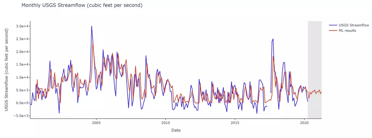
See the blue (past data) and red (ARIMA predictions) lines. This plot is far larger than our original time-series, given the scope of the data. By just observing the plot, we can see how closely ARIMA follows the past data. Let's now see the statistics.
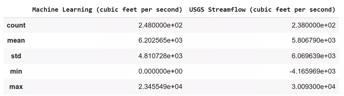
As we saw in the plot, the mean value for the past data (5806.79 ft3/s) is close to ARIMA's prediction (6202.56 ft3/s). However, we see some deviation between our minimum and maximum values, hence impacting ARIMA's accuracy in standard deviation.
All in all, in the case of Jacksonville, FL, we can conclude that a larger time frame results in a more accurate prediction.
Now, let us evaluate the statistics for Istanbul, Turkey in millimeters.
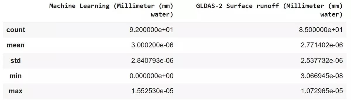
We can see that the model predicted a slightly greater mean (0.000003 mm) and standard deviation (0.0000028 mm) than the mean (~0.0000028 mm) and standard deviation (0.0000025 mm) of the past data.
This conclusion holds for other values present. The minimum and maximum values predicted by the tool are less accurate, but very closely resemble the past data for this location.
Given the closeness in accuracy between values, one could conclude that the tool gave an accurate prediction for runoff based on the inputted data for Istanbul, Turkey.
Again, just as in our streamflow plots for Jacksonville, FL, we can test ARIMA's ability to make predictions by specifying a larger timeframe.
- Note: since we must use the GLDAS dataset for Istanbul, remember GLDAS datasets get periodically updated and currently our tool extracts data only covering 2003-2023. So, for Istanbul we will use the dates of 2003-2023.
Here is the new time-series for runoff in Istanbul, Turkey. For Istanbul too, similar to our Jacksonville example, ARIMA performs with higher accuracy and precision when it is given a larger pool of data to learn from.
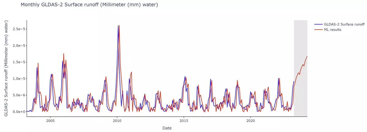
Take a close look at the gray sections in each of the time-series plots. Do you see how the duration of the past historical data used in ARIMA influenced its future predictions?
STEP 11 DOWNLOAD CSV FILE AND TIME SERIES TO YOUR PERSONAL COMPUTER
This step will allow you to download and store your desired results.
Results will always be downloaded as 'ML_results.' Ensure that you rename the file to reflect the correct location and date. Below is an example of the generated outputs.
You can see the time series plot that you just generated by simply selecting the PDF file within the "ML_Results" folder shown above. Clicking on this file will display the time series plot in a web-browser.
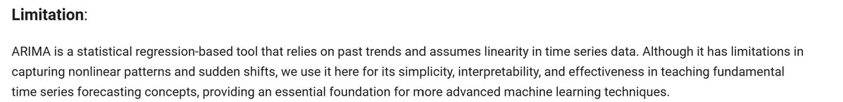
One final note: it is important to be aware that there are limitations to the ARIMA tool. In short, ARIMA is limited in its ability. However, it is an efficient statistical analysis tool for the purpose of this tutorial: introducing you to the many uses of machine learning and Artificial Intelligence in climate, water, and environmental assessments.
Great Job! Now you know how to run a Python code using Google Colaboratory, compare machine learning results to past historical data, and forecast future river discharge anywhere in the world using this web-based python tool!
Restart the tool to redo this exercise for any other location of your interest!
References:
- [USGS Streamflow data] U.S. Geological Survey, 2016, National Water Information System data available on the World Wide Web (USGS Water Data for the Nation), Retrieved from http://waterdata.usgs.gov/nwis/.
- [NASA GLDAS-2 surface runoff data] Li, B., H. Beaudoing, and M. Rodell, NASA/GSFC/HSL (2020), GLDAS Catchment Land Surface Model L4 daily 0.25 x 0.25 degree GRACE-DA1 V2.2, Greenbelt, Maryland, USA, Goddard Earth Sciences Data and Information Services Center (GES DISC), Accessed: May 15, 2024, 10.5067/TXBMLX370XX8
- Water Science School. (2019). Streamflow and the Water Cycle. U.S. Geological Survey. https://www.usgs.gov/special-topics/water-science-school/science/streamflow-and-water-cycle
- Fuqua School of Business. (n.d.). ARIMA Models for Time Series Forecasting. Introduction to ARIMA models. Retrieved from: https://people.duke.edu/~rnau/411arim.htm
- Data Science Batch of 2023. Chapter 1: AutoRegressive Integrated Moving Average (ARIMA) — Time Series Analysis Handbook. (2021). Asian Institute of Management. Retrieved from: https://phdinds-aim.github.io/time_series_handbook
- Livingston, E. (2004). The mean and standard deviation: What does it all mean?. Journal of Surgical Research, https://doi.org/10.1016/j.jss.2004.02.008