RisingSeas: An Online Python Tool to Study Sea Level Rise Projections and Trend Analysis
Introduction
Icebergs melt, seas surge, cities drown. Around the world, from Venice's sinking streets to Bangladesh's desperate plight, sea level rise has significant implications on coastal communities, ecosystems, and infrastructure. Additionally, ground subsidence (the natural settling or uplifting of the Earth's surface) may pose a compounding effect, increasing or decreasing the overall implication of sea level rise. To allow our communities to enhance their resilience planning, we need fast and efficient quantification of sea level rise and ground subsidence. But, the available data has often proven to be difficult to use and interpret. Specifically, downloading, processing, and analysis of sea level and ground subsidence data from diverse computer simulation models and remote sensors remain challenging. This tutorial will introduce a Python-based tool to automatically and instantly download, process, and analyze these data types.
To run the tool, you will access IPCC AR6 sea level projections and ground subsidence rates from GPS-based vertical land motions. Although we will use New Orleans, Louisiana as an example in this tutorial, the tool works for any coastal location in the world.
The tool has two unique features:
- It is an end-to-end workflow that performs all data discovery, download, pre-processing, and analysis tasks in a semi-automatic manner.
- Users can run this tool simply in a web browser without having to write Python codes or installing any software in personal computers.
Tool URL: https://colab.research.google.com/drive/13Dfk60BJm_2RV2q3r5SpGQpdfRkn9DMi
Video Demonstration: https://youtu.be/fapSiviXkJc
Conceptual Outcomes
- Users will learn how to apply coding to assess, analyze, and display sea level rise and ground subsidence data.
- The data derived from this tool will provide essential insights into the long-term trends of sea level rise until the end of the 21st century in any area of interest.
- Users will make real-world interpretations of climate change impacts by considering the combined influence of ground subsidence and sea level rise for any desired coastal location.
Practical Outcomes
- By completing this tutorial, users will learn how to develop and run python codes on a web-based platform in order to assess and analyze trends of sea level rise and ground subsidence.
- Users will get hands-on training on end-to-end discovery, integration, and analysis of complex vertical land motion data.
- Users will learn how to instantly analyze ground subsidence levels using python programming.
Time Required
It will take roughly 25 minutes to complete this tutorial. The required time may vary with the extent of the target area and the internet connection quality.
Instructions
Read this short tutorial carefully to set up your Google Colaboratory: Setting Up Google Colaboratory to Run Python Codes
Let's start by clicking on the link below: (This will open a python code in your computer's browser).
https://colab.research.google.com/drive/13Dfk60BJm_2RV2q3r5SpGQpdfRkn9DMi
Watch this instructional video to make yourself familiar with all the steps followed in this tutorial. You will see how we extracted the data to generate it for our desired location of interest. For this tutorial, we used the city of New Orleans, Louisiana to chart a trendline for sea-level rise throughout the 21st century. However, this tool will run for any location in the world.
You can executeevery step by merely clicking the play button or pressing "Ctrl+Enter". Relevant notes associated with each step are provided below.
If this is the first time you have accessed this tool, start by saving a copy of the tool in your Google Drive. This ensures that the user can start over or test out multiple different locations of choice. Then, start directly from Step 1.
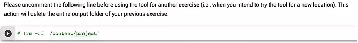
If this is NOT the first time you have used this tool, edit the following line of the code by deleting the "#" symbol, then press the play button. Pressing the play button will clear any data that you have generated with this tool in your previous attempts.
![[creative commons]](/images/creativecommons_16.png)
STEP 1: INSTALL PYTHON MODULES
Run the cell by pressing the "play" button.
STEP 2: IMPORT PYTHON MODULES
In this step, you are going to "call" the python packages/modules that you installed in the previous step.
Once you call them, those packages/modules will be ready to perform specific geospatial functions in the subsequent steps.
STEP 3: SELECT A LOCATION OF INTEREST
Run the first cell in this step to directly access the global map.
Proceed to the next cell, press play and pan over to your desired coastal area of interest. Select the circle marker to pin your location.
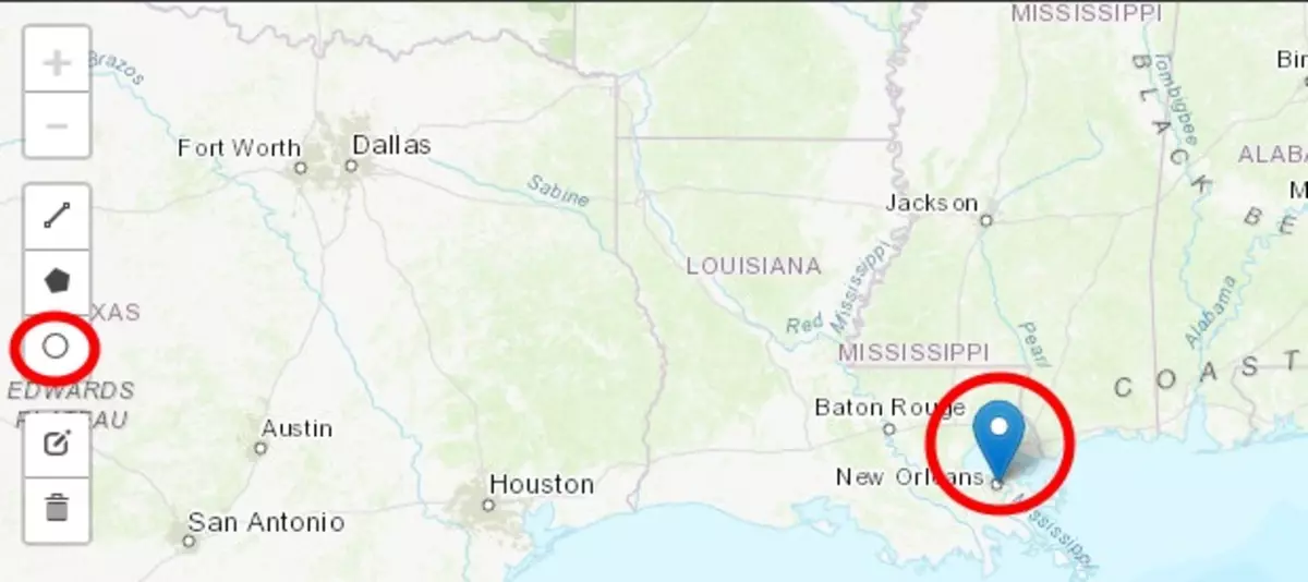
For this tutorial, our location of interest is New Orleans, Louisiana.
Finally, run the last cell in this step to auto-generate your coordinates for the selected location.

STEP 4: DEFINE FUNCTIONS
This step will instantly assess the location of interest.
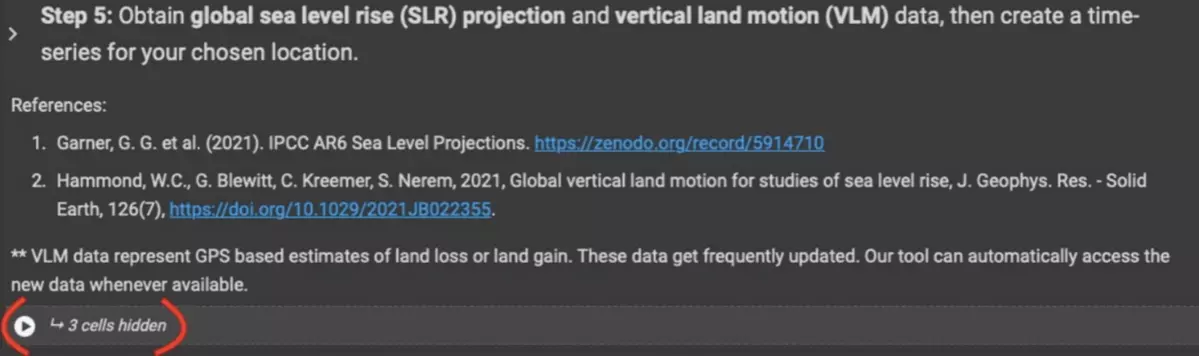
STEP 5: ACCESS THE DATA
This step will access the sea level projections and the global vertical land motion data for your desired location.
Please ensure all (3) cells have been called in order to access all the required data. This will then create a time series of sea level rise projections for the desired location.
In this time series, there are 4 different predictions, labeled "SSP 1-3" & "VLM."
- SSP(1): The term "SSP" refers to "Shared Socioeconomic Pathways," or different future scenarios based on the relationship between climate change and socioeconomic factors. SSP(1) implies a future scenario in which sustainable growth is principal in all human societies. In other words, SSP(1) is the "best case scenario."
- SSP(3): Colloquially called "The Rocky Road," SSP(3) predicts a future of slow economic growth, environmental degradation, and over-consumption. SSP(3) is characterized by high challenges in mitigation and adaptation to climate scenarios.
- SSP(5): Characterized by high challenges in mitigation, but low challenges in adaptation. SSP(5) assumes all human societies are driven by effective energy consumption and the sustainable practice of it. SSP(5) differs from SSP(1) in that all sustainable practices are purely economically-driven.
- VLM: As we know, VLM stands for "Vertical Land Motion," and represents a value for ground subsidence. An increasing VLM trendline indicates ground uplift, while a decreasing VLM indicates ground settling. VLM values are dependent on location, and can impact all SLR scenarios. For example, in regions that experience increasing rates of subsiding, SLR scenarios can compound or intensify.
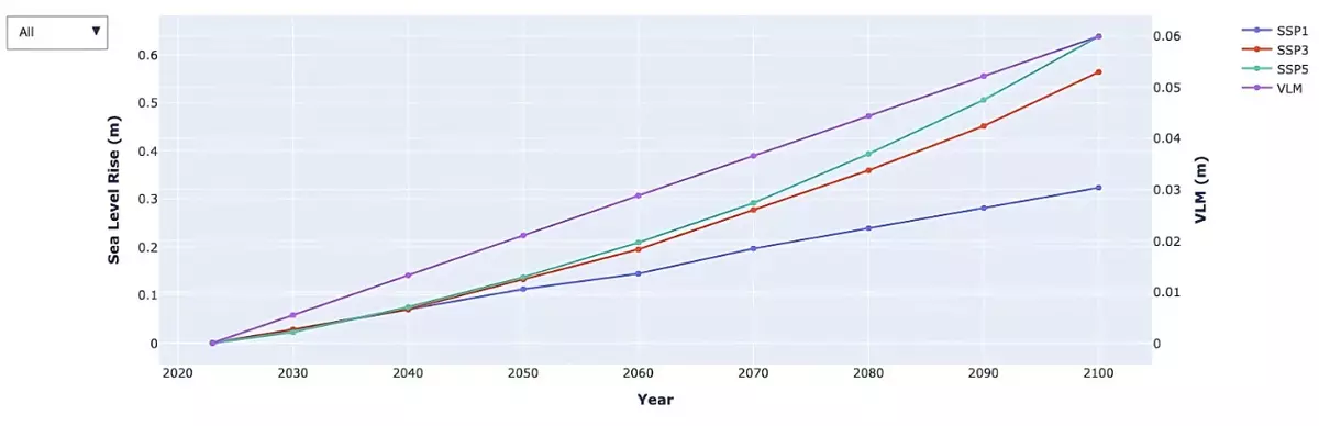
To gain a better understanding of the data, select an SSP or VLM from the drop-down menu on the left-hand side of the graph.
STEP 6: ANALYZE THE DATA
This step will prompt a response from the user. Identify which SSP you would like to use for this analysis. This step is case-sensitive, please reply exactly as one of the options seen below.

In this tutorial we will use SSP(5), which will generate a time series and a trendline analysis of the projected sea level rise. Note, the time series data generated in this step represents the combined influence of SLR and VLM. Think how an increasing VLM (ground uplift) will affect the net SLR, or vice versa.
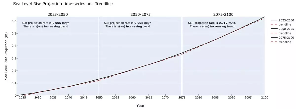
Above is a figure depicting the trendline analysis for New Orleans, Louisiana. Here are some key takeaways:
- "Trendline analysis" is a statistical term, and is used in figures such as above to display statistically meaningful data. If the total value for the data depicted is large, a trend is seen as significant, even if data points are scattered far from the trendline.⁴ A linear slope portrays a strong association between data points, and thus a trend is plausible. If no trendline can be drawn, there is a weak or no association between data.
- The figure above represents a positive linear slope throughout the 21st century (indicating an increasing trend). The graph is split into 3 parts: 1) 2023-2050, 2) 2050-2075, 3) 2075-2100. The trendline for New Orleans, Louisiana indicates that Sea Level Rise is predicted to rise at a rate of 0.005 m/year in part 1, 0.008 m/yr in part 2, and 0.012 m/yr in part 3.
STEP 7: DOWNLOAD RESULTS TO YOUR PERSONAL COMPUTER
This step will allow you to download and store your desired results.
Results will always be downloaded as 'SLR_Project'. Ensure that you rename the file to reflect the correct location.
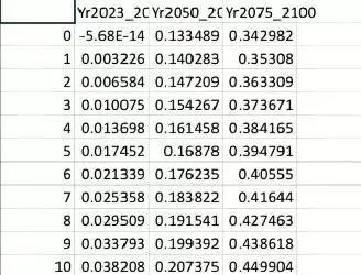
Below is an example of the generated outputs. You can see the time series plot that you just generated by simply opening the file in Excel. Clicking on this file will allow you to access the data used to predict the future sea level rise in your desired location.
Great job! Now you know how to run a Python code using Google Colaboratory, and project the future sea level rise using this web-based python tool. Restart this tutorial to generate a similar output for any other location of your interest!
References:
- Garner, G. G. et al. (2021). IPCC AR6 Sea Level Projections. https://zenodo.org/record/5914710
- Hammond, W.C., G. Blewitt, C. Kreemer, S. Nerem, 2021, Global vertical land motion for studies of sea level rise, J. Geophys. Res. - Solid Earth, 126(7), e2021JB022355, https://doi.org/10.1029/2021JB022355.
- Hausfather, Zeke. (2018). How Shared Economic Pathways Explore Future Climate Change. Carbon Brief, Clear on Climate. Retrieved from: https://www.carbonbrief.org/explainer-how-shared-socioeconomic-pathways-explore-future-climate-change/
- Bryhn, A. C., & Dimberg, P. H. (2011). An operational definition of a statistically meaningful trend. PloS one, 6(4), e19241. https://doi.org/10.1371/journal.pone.0019241