Part 2: Preprocessing Image Data³

Days 4 and 5 will guide you through a simulated research project. Most research conducted with digital images involves four phases: preprocessing, data collection, data analysis, and publication. Today, you'll get familiar with the data and prepare for the data collection workflow. While it's impossible to truly "start from scratch", you will work with raw, minimally-processed data. You will apply many of the skills you've learned throughout this course and will learn new tools to help relieve you of some of the tedium of data collection. The emphasis of today's work is on the overall process and workflow—preprocessing some of the data and getting everything ready to begin collecting actual data.

Background²

Investigation question: How has the the Arctic sea ice extent changed over time?

Minimum Sea Ice Extent - September

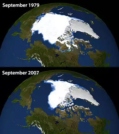
Sea ice - frozen, floating sea water - forms and melts with the seasons. If the ice grows thick enough, it does not melt completely, persisting from year to year. In the Arctic, the area covered by sea ice typically shrinks in the summer and expands in the winter.

Since the late 1970s, satellite data from NASA's Nimbus 7 satellite and the Defense Meteorological Satellite Program's SSMI (Special Sensor Microwave Imager) have shown that the average area, or extent, of Arctic sea ice remaining at the end of the summer melt has decreased dramatically, falling by over 8 percent per decade. In September 2007, the sea ice extent was at a record low.

The decrease in Arctic sea ice has widespread and significant environmental impacts, particularly on animal life. Polar bears hunt seals and other marine mammals on winter sea ice and fast on land during the summer melt. As the summer melt occurs earlier and earlier, the balance between the bears' feeding and fasting seasons is shifting. During the summer months the bears are forced to retreat to land and fast on their stored fat reserves until sea ice comes back in the fall. This has caused the average weight of female polar bears to fall by nearly 150 lbs. over the past 25 years. As females become lighter, their ability to reproduce and the survival of their young declines. Hungry bears are more likely to adapt to new habitats and move closer to human settlements as they seek food.

Download Images

To conduct this investigation, you need three different kinds of images. Set up a folder for this project and right-click (PC) or control-click (Mac) each of the file links to download the files to your computer.

1. A map of the Arctic, showing the different areas you want to analyze. Arctic Regions Map (Zip Archive 24kB Jul20 11)
2. Satellite images showing the extent of sea ice. (This is just one sample file. There will be others to download later.) September 2007 Arctic Data (Zip Archive 25kB Jul20 11)
3. A synthetic image to help us correct for the curvature of Earth and the inherent distortion of the map. Arctic Pixel Area (Zip Archive 312kB Jul20 11)

Unzip all three files to the project folder.

Examine the Images—Get the Big Picture

Before you start processing the images, you'll open each one to get a sense of the information it contains. The first file you'll look at is an example of the ice coverage data you'll be collecting and analyzing—Arctic_2007September.bin. The .bin file extension indicates that the file is a raw binary file. You will have to import it into ImageJ.

Sea Ice Data

• We have no metadata for this file, but we've been told that the image dimensions are 304 x 448 pixels. Before we even try to open the file, let's see what we can find out about it. What you do next depends on your operating system.
  • Windows – find the Arctic_2007September.bin file, right-click it, and choose Properties. Find the Size of the file (always use the number in parentheses). Close the properties window.
    Show me the file size, in bytes
    Hide
    The file size is 272,384 bytes.
    
    
    

    

    
    
  • Mac – In the Finder, locate the Arctic_2007September.bin file, click the file to select it, and choose File > Get Info. Find the Size of the file (always use the number in parentheses). Close the info window.
    Show me the file size, in bytes
    Hide
    The file size is 272,384 bytes.
    
    
    

    

    
    
• Working backward from our memory formulas, if I divide the memory, in bytes, by the width and height of the image in pixels, I should get the bit depth. (In bytes, since everything here is in bytes.) See if you can calculate the bit depth of this image so we can import it correctly.
  Show me the calculation
  Hide
  272384 / 304 / 448 = 2 That's two 8-bit bytes per pixel. This is a 16-bit image! When you do the calculation and you get nice, round, whole numbers you know you're probably on the right track.
  
  
  So, you know that it's a 16-bit image, but there are two "flavors" of 16-bit data: signed and unsigned, and we don't know which flavor this is. The best approach is to import the image both ways and see which version makes the most sense.
  
• Choose File > Import > Raw, navigate to the Arctic_2007September.bin file, enter the following settings to import the image as signed, and click OK.
  
  
  
  
• Repeat this process to import the same file as 16-bit unsigned.
  
  
  
  
  Show me what the images look like
  Hide
  The images look like this. The 16-bit signed version is on the left and the 16-bit unsigned version is on the right.
  

  

  
  
  
  
• Mouse around the image and look at the pixel values. The image is all about percentages of sea ice concentration. Describe the numbers you see and any associations they have with map features.
  Show me the answer
  Hide
  Signed (left) [entity 150 Land = -9999, Continent outlines = -10000, the "hole" in the middle (the satellite can't see that far North) = -50, ocean values range from 0 to 995.
  
  Unsigned (right) [entity 150 Land = 55537, Continent outlines = 55536, the "hole" in the middle (the satellite can't see that far North) = 65486, ocean values range from 0 to 995.
  
  .
• Based on these values, which image do you think has the most logical values? (Hint: No Data values are often negative numbers.)
  Show me the answer
  Hide
  This is a 16-bit signed image.
  
  
• If the ocean values range from 0 to 995 and they are supposed to represent percent ice cover, what do you think the values mean?
  Show me the answer
  Hide
  The percentages were recorded to the nearest 0.1%, but 16-bit images can't encode decimals, so they multiplied the values by 10. Thus, 995 = 99.5% ice cover.
  
  
• Close the 16-bit unsigned image.

Arctic Study Regions

• Open the Arctic_Regions.tif image.
Hey—an image that's obvious for once! Clearly, this is a map showing the seven arctic research areas. The map came from a PDF file that was then saved as a TIFF file.


• Use the rectangular selection tool to measure the approximate width and height of the map. Notice anything about the map's dimensions?
  Show me the answer
  Hide
  The map dimensions are about 304 x 448, the dimensions of the data images.
  
  
• Later, you will crop out this map and process it to create ROIs for each of the seven study regions.

Arctic Pixel Area

• Check the size, in bytes, of the Arctic_Pixel_Area.bin file. Do the math—what is the bit depth of this image?
  Show me the bit depth
  Hide
  The file size is 544,768 bytes. Dividing by the width and height: 544768 / 304 / 448 = 4 bytes/pixel. This is a 32-bit image! Most 32-bit images are 32-bit real (floating point) format, so go with that.
  
  
• Import the file as a 304 x 448-pixel raw file using the bit depth you just calculated.
• Mouse around the image and look at the pixel values. A little different, aren't they? How do you read these values?
  Show me
  Hide
  The image looks like this, and the pixel values are so large they are displayed in scientific notation. For example, the value of pixel 189,47 is 5.01185856E8. The E8 means x108 or "hundred million". Thus, the value of this pixel is about 5 hundred million!
  
  
  

  

  
  
  The significance of this image is interesting. Please read carefully...
  
  

  Pixel Value = Area (Correcting for Distortion)

  This is a synthetic image. It wasn't "taken" like a photo or "drawn" like a picture. Rather, it was calculated by a computer. The image was produced specifically for this data set. What does it "show"?
  
  The sea ice images were produced in a polar map projection. An important limitation of projected images is that the areas they depict are distorted. As you get farther from the center—the pole—the image gets stretched out. As a result, as you move away from the pole, the area represented by a pixel gets smaller and smaller. This may be counterintuitive, but it's true. That means you can't simply set a scale on this image and make area measurements. But, if you can identify the pixels you're interested in, you can get their combined area by adding up all their pixel values! (Neat trick, isn't it?)
  
  In this image, the value of each pixel represents the actual area on the ground that the pixel represents, in square meters. A histogram reveals that these areas range from a minimum of 379741248 square meters to a maximum of 657685824 square meters. (A square kilometer is 1,000,000 square meters, so this translates to a range of about 380 square kilometers to about 658 square kilometers per pixel.)
  
  The data collection will work like this: you'll threshold and auto-outline the sea ice images to identify an ROI where the ice is, and save the ROI to the ROI Manager. You'll intersect this ROI with the ROI for each study area (that you will create from the processed map). Intersecting sea ice with study area produces a new ROI you could call sea ice in study area. To measure the AREA of the sea ice, you will then transfer the sea ice in study area ROI to the Arctic Pixel Area image, and measure. The measurement you're interested in is NOT the area of the ROI, but the sum of all the pixel values (the true pixel areas encoded as the value of each pixel). The name for this measurement is integrated density.
  
  This information is pretty "thick", so don't worry if it isn't perfectly clear now, but come back here later to read and re-assimilate the main ideas.
  
  
• Save the Arctic sea ice (Arctic_2007September) image to your project folder in TIFF format.
• Save the Arctic pixel area image to your project folder in TIFF format. The next time you use these images, open the TIFF versions so you don't have to mess with the importing process.
  

Processing the Study Areas Map

Now that you have a clue about the images you'll be working with, there's one bit of pre-processing left to do. You need to turn the study area map image into something you can use for selecting the regions in the sea ice images. This will require two steps: cropping the map out of the middle of the image, and removing the black lines from the image.

Cropping out the map

• Zoom in on the map image and find the coordinates of the pixel in the upper left corner of the map border.
  Show me the coordinates
  Hide
  The coordinates are 109,275.
  
  
  

  

  
  
• Choose Edit > Selection > Specify and enter the width and height of the required image (304 x 448) and the coordinates of the upper left pixel, then click OK. This will select the map area.
  
  Show me
  Hide
  

  
  
• Choose Image > Duplicate to create a new image window from the selection.
• Save the cropped image as a TIFF file.

Removing the black lines

The black lines on the map image will interfere with selecting and creating an ROI for each study region. Now you will use digital filtering techniques to remove these lines. In digital filtering, pixel values are analyzed and modified (or left alone) based on their relationship with the surrounding pixel values. For example, the median filter replaces the value of every pixel with the median (middle) value of the pixel's 3 x 3 neighborhood. (In other words, the pixel and its eight neighbors.)

• Experiment with the different filters under the Process menu. You are looking for a process that will remove the black pixels without changing the rest of the image. After applying a filter, choose Revert so you can test the next filter. Some filters provide control over different values and parameters.
• You may have found a filter that does exactly what's required. If not, one solution is shown in the "show me" below.
  Show me how to filter out the black lines from the map image.
  Hide
  The filter used here is the Remove Outliers filter, in the Noise submenu. As you test different values for the Radius and Threshold, turn on the Preview option so you can see the results of your changes. The settings shown produce good results.
  
  
  

  

  
  
• The map is now ready to use. Save your cleaned-up map in TIFF format, with a new name.

Creating Study Area ROIs

To process the data, you need to create a set of ROIs for the different Arctic study areas. Using the original color map of the Arctic Regions with the legend, choose four of the nine labeled areas to study. These instructions will guide you through the process of creating the ROI for the Arctic Ocean study area. It will be your responsibility to create ROIs for three additional study areas and use the ROIs to measure the total area of each chosen study region. To create the Arctic Ocean ROI:

• Choose Image > Adjust > Threshold to open the Threshold Color window.
• Consult the legend and find the Arctic Ocean study area. (Hind: It includes the pole.)
• In the Threshold Color window, adjust the channel sliders until ONLY the pixels in the Arctic Ocean study region are highlighted.
  
  
  
  
• Click the Select button at the bottom of the Threshold Color window.
• Choose Edit > Selection > Add to Manager to add this selection to the ROI manager.
• Rename the ROI in the ROI Manager to "Arctic Ocean".
• Repeat this process to create ROIs for at least three additional study areas.

  A note about Color Thresholding

  The color thresholding tool, as advertised, is "experimental". As such, it can be quirky and jumpy at times. If you get lost, try clicking the Original button at the bottom of the window and start over. If you are working in the HSB (hue, saturation, and brightness) color space, which I suggest you do in this case, leave the saturation and brightness range from 0 to 255 and adjust only the hue (color) range to highlight each study area in turn. The display may suddenly switch to binary (black on white), but as long as you can isolate a study area and click Select you should be good to add the selection to the ROI Manager.
  
  If Threshold Color takes to you the point where you want to throw your laptop off a cliff or pull your hair out, feel free to "adapt" to the situation and use a different tool or technique, such as the Wand (auto-trace) tool. The downside of other techniques is that they don't handle non-contiguous regions of pixels as easily as thresholding. You may have to auto-trace one area, then hold down the shift key as you trace additional areas with the same color.
  
  

Save the ROI file

Now that you have created ROIs for your study areas, save them to a file so you can use them any time you need them.

• Deselect all of the ROIs in the left-hand column of the ROI Manager.
• Click the More button at the bottom of the ROI Manager and choose Save As from the pop-up menu.
• Name your ROI file Arctic_ROI.zip and save it into your project folder. All of your ROIs will be stored in the zipped file. You do not need to unzip this file. Any time you need these ROIs, simply drag and drop the .zip file onto the ImageJ toolbar.

Your Assignment: Reapply Regions of Interest To a New Image and Measure

This assignment is basically a check to make sure all the pieces you have prepared so far are working together correctly. Please submit what you have, whether it's working perfectly or not.

1. Use the ROI Manager to select and measure the area of each of the four study regions you chose on the Arctic_Pixel_Area.tif image, in square meters. Remember that you are NOT measuring the area of the selection in pixels, you are measuring the Integrated Density, which you need to turn on in the Set Measurements dialog box.
2. Take a screen shot showing your image with one or more ROIs applied, the ROI Manager window, and the Results window showing your four measurements, and post it to the Part 2: Share and Discuss Page.

Source