For the Instructor

These student materials complement the Modeling Earth Systems Instructor Materials. If you would like your students to have access to the student materials, we suggest you either point them at the Student Version which omits the framing pages with information designed for faculty (and this box). Or you can download these pages in several formats that you can include in your course website or local Learning Managment System. Learn more about using, modifying, and sharing InTeGrate teaching materials.

Unit 3 Reading: Earth's Energy Balance

by Louisa Bradtmiller, Macalester College, and Kirsten Menking, Vassar College

In this lab we will explore Earth's radiation budget using several versions of a simple climate model often referred to as a "layer model." Earth receives energy from the sun, some of which is reflected back to outer space but most of which is absorbed near the surface. The absorbed energy is then re-radiated upward from the surface where it is then absorbed and re-radiated by the atmosphere or goes nearly directly to space. An imbalance between incoming and outgoing energy results in a change in average global temperature until equilibrium is restored. We will start with a very simple model in which all energy is absorbed (no reflection) and end with a model that can closely approximate Earth's temperature record for the last 1000 years.

Radiative equilibrium models

Radiative equilibrium models are based on the starting assumption that Earth is a "black body," which means that it absorbs and re-radiates all energy incident upon it from the sun; in other words, flux in = flux out. This assumption allows one to calculate the equilibrium temperature for Earth from the Stefan-Boltzmann Law, which states that the energy given off by a black body is a function of its temperature:

` E = sigmaT^4 `

where E is the energy given off by the black body, ` sigma ` is the Stefan-Boltzmann constant (5.67×10^-8W/m²K⁴), and T is the temperature in Kelvin. Since a black body gives off as much energy as it absorbs, incoming energy must be equal to outgoing, and thus the equilibrium temperature can be determined by equating the energy absorbed from the sun (S₀) to the right-hand side of the equation above:

` S_0 = sigmaT^4 `

S₀ has a measured value of 1366 W/m² at Earth's position in the solar system. Before we can solve this equation, however, there is one final aspect that we must consider. Figure 1 shows the geometrical difference between the way energy is absorbed from the sun and how it is re-radiated from Earth. Specifically, sunlight is intercepted in space by a disc with the area of a circle with the radius of Earth. Energy is radiated from a sphere with the same radius. Therefore, we see a factor of 4 difference between incoming and outgoing radiation. Given this, the radiative equilibrium temperature for the planet can be calculated using a slightly modified version of the Stefan-Boltzmann Law:

` S_0 (pi r^2) = sigmaT^4(4pi r^2)`

A related law, known as Wien's displacement law, relates the wavelength of peak energy emission to the black body temperature in Kelvin:

` lambda_(peak) = 2897/T ` (units of wavelength are micrometers)

This tells us at what wavelengths a body will emit most of its energy, and therefore whether that energy is likely to interact with gases in the atmosphere, which only absorb at specific sets of wavelengths. Wien's law tells us that Earth radiates in the infrared part of the electromagnetic spectrum, right at the wavelengths where gases like CO₂, H₂O and CH₄ absorb most strongly.

Imagining the atmosphere as a "layer"

While a simple black body assumption for Earth gets us pretty close to being able to calculate our planet's average surface temperature, we can improve our model by adding a layer to represent the atmosphere (Figure 2).

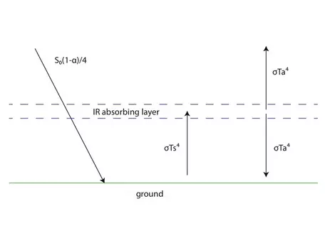
For starters, we make the same assumptions about the layer that we did about Earth; that is, it absorbs all incoming energy from Earth, and re-radiates all energy it receives. Because it is slightly above Earth's surface however, it can radiate both up to space and down to Earth (as opposed to Earth's unidirectional upward radiation). Note that in this simplified model, the atmosphere layer does not absorb incoming energy from the sun; instead solar energy makes it all the way to the surface undisturbed. This is a reasonable approximation because incoming solar energy occurs primarily at wavelengths in the UV spectrum that are mostly not absorbed by the components of the atmosphere. Given the temperature of the sun (~5700K), can you use Wien's law to prove to yourself that this is true?

Figure 2 also contains a new symbol. The symbol ` alpha ` represents albedo, or reflectivity, and is simply a ratio (decimal) between 0 and 1, with 0 representing no reflection and 1 being total reflection from the surface. Using Figure 2 you could now write three different radiative equilibrium equations (flux in = flux out). You could write one for the surface, one for the atmosphere layer, and one for the whole system. Solving these would allow you to calculate the temperatures of the atmosphere and/or the surface.

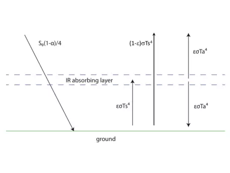
Emissivity

There are, unsurprisingly, many oversimplifications in our model so far. More specifically, there are a number of processes not represented by our one-layer atmosphere. For example, the atmosphere does absorb a small amount of incoming radiation (thankfully in the harmful-to-humans UV part of the spectrum!). In addition, there are mechanisms besides radiation responsible for moving heat or energy from the surface to the atmosphere, such as convection and conduction. Finally, there is a small fraction of radiation (at wavelengths not absorbed by CO₂ and other greenhouse gases) that escapes directly from Earth's surface to space. One option in modeling the climate system would be to include these processes individually and explicitly. Another option is to approximate them by introducing another term into our equations.

This term, called the emissivity (ε), is described by a ratio between 0 and 1, with 0 representing an object that does not re-emit any incoming radiation, and 1 representing an object that re-emits all incoming radiation. Figure 3 shows how we can incorporate emissivity into our layer model. When we do so, we can come very close to calculating Earth's average surface temperature.

Sunspots

Another simplification of the actual solar-Earth energy balance system that we have made so far is to assume that the amount of incoming radiation from the sun is constant over time when, in fact, it varies slightly. Sunspots are temporary dark spots on the surface of the sun. Solar radiation increases slightly with more sunspots, since the margins of the spots are much hotter than the surrounding surface, and thus actually emit more energy overall. The number of sunspots varies in cycles of approximately 11 years, though the magnitude of the peaks also varies through time.

Figure 4 shows observations of the number of sunspots over the past ~400 years. If we want to know about variations in sunspots (and therefore incoming solar radiation) farther back in time, we can look to records of isotopes such as ¹⁴C or ¹⁰Be that are produced when incoming solar radiation interacts with atoms in the atmosphere. You will encounter some of these data at the end of today's lab exercise.

Tips on radiative equilibrium modeling in STELLA

Casting the black body Earth problem in STELLA terms requires the creation of a reservoir into which the incoming solar energy flows and out of which the emitted infrared energy flows. Since the flows of energy into and out of this reservoir are measured in W/m², the reservoir itself contains Joules/m² (1 Watt = 1 Joule/second). To make the problem more tractable, it is easier to conceive of the flows as coming in Joules per year, which requires multiplying the solar constant by the cross-sectional area of Earth and the outflow from the Stefan-Boltzmann law by Earth's surface area (see Figure 1). In addition, both flows need to be multiplied by the number of seconds in a year. As a result of multiplying the flows by these areas and by seconds/year, the reservoir contains only Joules of energy. This allows a straightforward calculation of planetary temperature by dividing the energy contained in the reservoir (J) by its heat capacity (J/K).

In the model in this exercise, we follow the lead of Arthur Few (1996), and conceive of Earth's surface as a "swamp" of water 1 meter deep. The swamp assumption allows the heat capacity (c) to be calculated from the following:

` c = d * A * rho * sh `

where d is the depth of water in meters, A is the surface area of Earth (` 4pir^2 `), ` rho ` is the density of water, and sh is its specific heat.

Because this model reflects equilibrium (steady state) between inflowing and outflowing energy and because the inflows remain constant, the ultimate temperature reaches the same value regardless of layer thickness, density, and specific heat. In other words, one achieves the same result whether one uses a 10 cm-thick layer of water or a 20 m-thick layer of rock. Where the type of material is important is in the time required to reach steady state. The smaller the heat capacity of the material, the more quickly the surface temperature reaches the steady state value.

Once our model is created, we can experiment with the impacts of different climate forcings, such as the variations in solar radiation already described. A climate forcing is any influence on climate that originates outside the climate system. There are hundreds of climate forcings, but only a few that have relatively significant impacts on Earth's surface temperature. We will use records of four different forcings over the last 1000 years (Figure 5) to drive our model, and then compare the model temperatures to observed and reconstructed temperature data for the last millennium. The four forcings included in the model are:

Solar variability — as described above, sunspots change slightly the amount of incoming radiation from the sun.
Volcanic eruptions — large volcanic eruptions put small particles high into the atmosphere that reflect incoming radiation for up to a few years until they eventually fall to Earth.
Aerosols — this also refers to small particles high in the atmosphere, but specifically to those that are the result of anthropogenic (human) industrial activity.
Greenhouse gases — greenhouse gases occur naturally in the atmosphere, and your model incorporating emissivity accounts for the "natural" greenhouse effect. The greenhouse gas forcing mentioned here refers to the additional greenhouse gases that have been emitted as a result of anthropogenic industrial activity or deforestation.

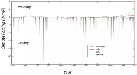
All of the forcings (found in an Excel file accompanying the exercise) are in units of W/m². In order to incorporate them into your model, you will need to think first about which flows they will affect. Note that these forcings are deviations from the "normal" model, so they will not replace, for example, incoming solar radiation; they will just modify it. To make the forcings compatible with the rest of the model, it may be necessary to multiply them by seconds/year, although this will depend on how you set things up.

References

Arthur Few, 1996, System Behavior and System Modeling, Sausalito, CA: University Science Books, 100 p.