Part 3—Convert Map Data to Numerical Data

There are 23 maps for each species of plant listed. The oldest map represents pollen distribution 21,000 years ago, followed by maps every 1000 years. An additional map of plant distribution is available at 500 years ago.

You can investigate change across any time span that interests you and you can analyze images at time intervals of 1000 years or greater. For example, you may want to study changes in the distribution of a plant between 10,000 and 5,000 years ago, tracking change at 1000-year intervals; for that investigation you'd need to analyze 6 different maps. For illustrative purposes, our example in this chapter will track distribution of the Alder from present time back to 21,000 years ago, but will only analyze every third image file.

1. Choose your plant species and the time interval.
2. Copy the maps (the .gif files) of the selected plant for the chosen time interval from the Images folder to your newly-created folder ("Pollen" or other folder created in Part 2.)

1. Launch the Analyzing Digital Images software by clicking on AnalyzingDigitalImages in the Pollen folder.
2. Choose File > Open Picture and navigate to the map of the present plant distribution for your species of interest (for example, ald0000.gif, if you have chosen the Alder as your plant species to investigate).
   
   
   
3. The Pollen Viewer maps will not be calibrated because the map projection creates a distortion of the pixel size with latitude. In the window titled Select Method to calibrate Pixel Size, select None.
   Show me how
   Hide
   

   
   
   
4. The first image of Alder distribution will display.
   Show me what it looks like
   Hide
   

   
   
   
5. Define your geographical area of interest by choosing the Spatial Analysis tab.
Show me how
Hide
1. Choose the Spatial Analysis tab.
   
   
   
   
6. Use the Rectangle Tool or Polygon Tool to select your area of interest. In this example, the state of Alaska is selected as the geographical area of interest.
Show me how
Hide
1. Choose the Rectangle Tool or Polygon Tool to define your area of interest.
   
   
   
   
2. If your area of interest is rectangular, select the Rectangle Tool and click and draw a rectangle on the map; the corners of the rectangle can be modified once drawn.
   
   
   
   
3. If your area of interest is irregular in shape, select the Polygon Tool and click each location of the polygon corner on the map, with the last click being close to the first corner (the software recognizes this at the closing of the polygon). Each polygon may have up to 20 corners and any corner may be modified by selecting the corner and dragging it.
   
   
   
   
   In this case, the polygon gives a much better approximation of the area due to Alaska's irregular border. Click on the image to get a larger view.
   




Practice selecting your area of interest by creating rectangles and/or polygons on the map. Only one "area" can be selected at a time on the map. Define your area until you are satisfied with its outline.

For help locating the exact geographic location of your study, you may want to consult these maps of North America.

In this step, you will isolate pixels by color, as they represent the different percentages of your species. These color masks will allow the software to count the number of pixels that represent your species in different time frames.

In this step, ald7000.gif is used as an example because it provides six different colors: gray, light green, dark green, black, blue, and white. The blue corresponds to blue ice, which doesn't appear until around 7000 years ago. If you choose an image "newer" than that, you will not be able to create a mask for the blue ice.

1. Click on the Mask Colors button.
2. Select the color(s) you wish to mask by dragging a box of any size within the desired color; it is easiest to start with the color of the lowest abundance. In this example, a box is drawn over the mid-west to easily capture the gray pixels. Note: This box will not alter the area of interest you selected on the Spatial Analysis window.
   
   
   
   
3. From the main menu, choose Save Color Masks > Save Color Mask 1.



4. Name the color mask. Specify a name that has meaning, such as the range of abundance (0-5%), the color (gray), or both and click Done.



5. Click on Apply Mask-TEST 1. You will see a message on your screen while the data is converted.



Show me how the map looks with the mask applied
Hide



Show me information about color masks
Hide
A color mask highlights (in black) all of the pixels in an image that are of a chosen color or range of colors, and it hides all other pixels. The benefit of isolating selected colors in this way is that the Analyzing Digital Images software can then count the pixels of the selected color, which allows the user to measure the extent of various colors in an image or track changes for a particular color across a time series of images. In the images below, the light gray in the image on the left was selected. The resulting color mask is shown on the right. Every pixel that was light gray has been colored black (the mask), and every pixel that was not gray is now white. The software can now use the mask to count the number of pixels that were gray in the original image and that were also within your selected area of interest.




6. Repeat steps 2, 3, 4, and 5 above until you have created a mask for each color you wish to study. In this example, six color masks have been created. Depending upon your species of interest and the time series that you have chosen, your images may look differently.
Show me the six color masks
Hide
The example uses the following six masks:
• Gray 0 - 5%
• Light Green 5 to 20%
• Dark Green 20 to 40%
• Black 40 to 100%
• Blue ice
• White - no data

If you make a mistake in the color range or the name of the color mask, just repeat the Save Color Masks function.

7. After you have identified and saved each of the color masks, save your selections to a file; select Save Color Masks > Save Color Masks to File. Save this file to your "Pollen" folder; this file will be recalled and used in the next step.

In this example, the species Alder has been selected and the spatial area has been defined as the state of Alaska. In this step, select every third image to analyze the data trends—ald00000.gif, ald03000.gif, ald06000.gif, etc. up to ald21000.gif. Images should be processed sequentially with respect to time; start with the present and progress to the oldest map. Note: you may choose to select a greater number of images later on if you decide to do further analysis.

1. Choose File > Open Picture to open your desired map, the one from the "present". You may see a window asking you to Keep settings? Click the Keep Settings button.
2. Check to see if your defined color masks display in the Apply Color Masks feature under the main menu. If they don't, choose Save Color Masks > Recall Color Masks from File and choose the color file you created in step 3 above.
3. Choose Apply Color Masks > Apply Color Mask 1. On this example, Color Mask 1 is named "Gray 0 - 5."
   
   
   
   
The gray pixels within the color mask turn black, and those outside the range turn white. The window will automatically go to the Mask Colors window so you can check to see if it is what you expected.
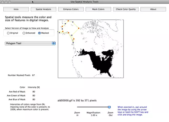
4. If the mask looks correct, select the Spatial Analysis button. Do NOT change the spatial tool used to create your selected area! This needs to remain the same throughout the data collecting. In the image below, the software has counted the number of black pixels in the selected area.
   
   
   
   
Show me the whole sequence of the color masked maps
Hide
Alder - Present - Color Mask 1; Gray 0 - 5%


Alder - Present - Color Mask 2; Light Green 5 - 20%


Alder - Present - Color Mask 3; Dark Green 20 - 40%


Alder - Present - Color Mask 4; Black 40 - 100%


Alder - Present - Color Mask 5; Blue Ice


Alder - Present - Color Mask 6; White, no data



5. Next, you will measure the number of black pixels, within your defined geographical area. From the main menu, choose Measurements > Save Measurement, or type CTRL-M (PC) or Apple-M (Mac).
   
   
   
   If you haven't opened a file to save your data, you will be asked to create one. If you are adding to an existing file, use this file name; otherwise, create a unique name to remember your work. In this example, the file was named "AlaskaAlders.txt".


6. A measurements information page will display. You may enter information in the Additional Data to be saved and Comments fields, or they can be left blank. Options include: the years before present, the color being masked, the range of abundance represented by the color, etc. The data displayed in the text boxes will be saved automatically—plus the name of the map being processed and the percent of pixels that are masked within the selected area. This last measurement is what you will be using later for analysis.
   
   
   
7. Repeat steps 1 - 6 for each color mask on each of your images. In this example, there are 6 color masks and 8 images. All 48 measurements and their corresponding information will be saved in the AlaskaAlders.txt file.