Part 3—Generate a Time Series Plot of Temperature
Step 1 – Launch EdGCM
 Launch EdGCM by double clicking the icon (alias pictured to the right) in the EdGCM folder. The application will load. The tool bar window will appear. It is from this toolbar window that the user controls the software. The buttons in this window will change depending on the active window.
EdGCM toolbar

- On the left side of the Toolbar window, select Modern_PredictedSST in the toolbar Run List. Note: to "select" a file in EdGCM, single click on the name.
Modern_PredictedSST is a simulation that demonstrates what future climate would be like with no increase in greenhouse gases or any other variables, such as solar luminosity. This is the baseline, or "control run," for any climate change experiments.
-
 Toolbar window
 In EdGCM, use the drop down Window menu and select, Analyze Output or, use the Analyze Output button at the top of the Toolbar (pictured right).
- In the Analyze Output window, click on the Time Series tab near the top of the window, then click the button called Time Series in the bottom left hand corner of the window.
Analyze output window.

Note: if this step has been done previously, the Time Series button may be grayed out (i.e inactive), if so progress to the next step.
Note: This step runs a program that takes a little while on slower computers. To save time the teacher might do this step before class.
Once this button is clicked a new window will open showing you that the program is running a Time Series.
- In the list of variables in the center section of Analyze Output window, select the check box next to Surface Air Temperature then click the Extract button in the center bottom part of window.
Note: If the extract button is grayed out you have not yet computed the Time Series; it is described in the previous step.
- In the right hand column of this window, under view images, select SRFAIRTMP (Surface Air Temperature) and click the View button below that column. This will launch EdGCM's scientific visualization application or EVA, and open EVA's Data Browser window. The Data Browser will list one simulation in the File column, Surface Air Temperature in the Variable column, and 5 items in the Time or Region column. Confirm that you have these items and then ignore this window while you import a second data set.
- In EVA data browser open the preference window. Under the Plot Window menu de-select (turn off) the auto produce plots on file open. Close the preference window.
Screen shot of preferences window with the preferences checked.

Step 2 – Select the IPCC_A1FI_CO2 Simulation for Comparison
- Return to EdGCM and select the IPCC_A1FI_CO2 simulation, by single clicking on the name in the Run List.
IPCC_A1FI_CO2 is the climate change experiment where the greenhouse gas quantities increase gradually as the model runs. These greenhouse gas "trends" have been predicted by scientists and economists working for the Intergovernmental Panel on Climate Change and are based on projections of how much energy humans will use in the future.
- Extract the data for analysis by repeating the steps numbered 4-6 from Step 1 with IPCC_A1FI_CO2 simulation.
- On the left side of the Toolbar window, select IPCC_A1FI_CO2 in the toolbar Run List. Note: to "select" a file in EdGCM, single click on the name.
- In EdGCM use the drop down Window menu and select, Analyze Output
or, use the Analyze Output button at the top of the Toolbar.
- In the Analyze Output window, click on the Time Series tab near the top of the window, then click the button called Time Series in the bottom left hand corner of the window.
Note: if this step has been done previously, the Time Series button may be grayed out (i.e inactive), if so progress to the next step.
Note: This step runs a program that takes a little while on slower computers. To save time the teacher might do this step before class.
Once this button is clicked a new window will open showing you that the program is running a Time Series.
- In the list of variables in the center section of Analyze Output window, select the check box next to Surface Air Temperature then click the Extract button in the center bottom part of window. Note: If the extract button is grayed out you have not yet computed the Time Series, it is described in the previous step.
- In the right hand column of this window, under view images, select SRFAIRTMP (Surface Air Temperature) and click the View button below that column. This will launch EdGCM's scientific visualization application or EVA, and open EVA's Data Browser window. The Data Browser will list two simulations in the File column, Surface Air Temperature in the Variable column, and 5 items in the Time or Region column. Confirm that you have these items and then ignore this window while you import a second data set.
Step 3 – Plot your Selections
- In EVA data browser, select the two SRFAIRTMP files listed in the 1st column, by clicking with the shift key held down. Then select Surface Air Temperature (2nd column), and select Global (3rd column)
EVA data browser with selections.

- Click the button on lower right to Plot All.

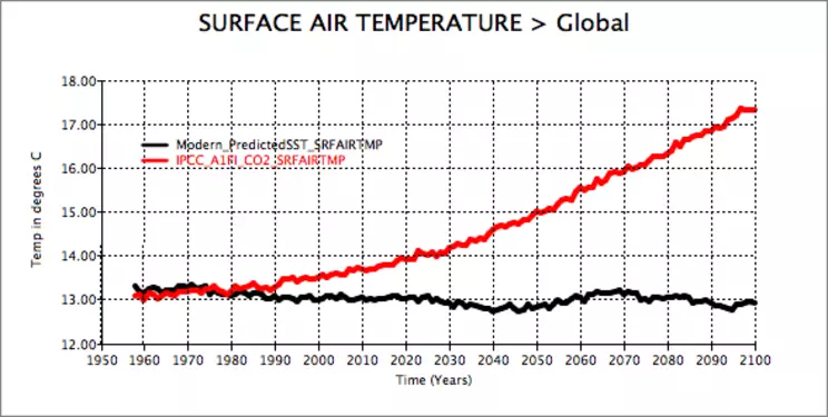
The program may hesitate briefly as it prepares an image (graph), then it will plot the two temperature trends on the same graph.
Completed temperature graph.
Annual Surface air temperature MAP using MPSST
![[creative commons]](/images/creativecommons_16.png)
Provenance: Betsy Youngman, none
Reuse: This item is offered under a Creative Commons Attribution-NonCommercial-ShareAlike license http://creativecommons.org/licenses/by-nc-sa/3.0/ You may reuse this item for non-commercial purposes as long as you provide attribution and offer any derivative works under a similar license.
Step 4 – Finalize your Graph
- Finalize your first graph using the instructions below.
- Click and drag the legend to relocate it to the upper left hand corner.
- Click to turn on horizontal and vertical grids.
- Clean up the legend, by changing the colors and font size.
- Add a title "temperature in degrees C" to the Y axis.
- Answer the following questions about the graph:
- Save your graph for future reference. Give it a unique name that describes the graph.
Step 5 – Use EdGCM to Calculate the Difference Between Simulations
- In EVA data browser, use the pull down the differencing menu, located in the lower right hand corner, and select the two files to compare. Subtract the control run (modern_predictedSST) from the experimental run (IPCC_A1FI_CO2).
Examine the differencing menu pictured below. Data 1 is the first graph generated and Data 2 is the second. The order of the list itself is determined by the order the data was added to the browser. In this example the equation will be (data 2- data 1) or (IPCC_A1FI_CO2) - (modern_predictedSST).

- If needed, click the Plot All button.

Note: In most cases the plot will automatically be generated.
- Finalize your graph.
- Click and drag the legend to relocate it to the upper left hand corner.
- Click to turn on horizontal and vertical grids
- Clean up the legend, by changing the colors and font size.
- Add a title, such as "difference in temperature in degrees C" to the Y axis
Note the units on the difference graph are not the same as on the original graph. They are degrees of difference between the first simulation and the second. This "difference" is also known as an anomaly.

- Give your graph a unique name that describes the graph and save the graph.
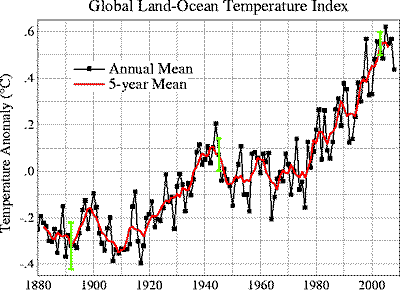 Line plot of global mean land-ocean temperature index, 1880 to present. The dotted black line is the annual mean and the solid red line is the five-year mean. The green bars show uncertainty estimates. Note: This is an update of Fig. 1A in Hansen et al. (2006)
- Compare your graph of modeled data with the one from NASA observed data, shown right. Note: the axes on the two graphs differ (1880-2010 vs. 1950-2100 on X axes) because the observational record is different from the years simulated with the model. On the Y axes the scale is much larger on the modeled data than the observed data. Make sure you are comparing data where the two overlap. Optional: read more about this graph Global Annual Mean Surface Air Temperature Change.
Answer the following questions about the two graphs:
- How does the modeled data IPCC_A1FI_CO2 compare with the observational data? Are there years where they are the same? different?
- By how much does the temperature change in each graph between the years 1960 and 2000?
- What other information do graphs of average global temperature leave out?
The two graphs, observed and modeled show the same results in the years 1960 -2000. The amount of change is slight, less than 1 degree centigrade. A graph of global temperature average does not show what is happening in any one particular location. In some areas, such as the Arctic these changes are much more extreme, hence the importance of local monitoring efforts.
- Optional: Compare your graph of modeled data using EdGCM to other graphs of temperature trends from the NCAR climate model animation (more info) . Note the similarities and differences in the 4 trends. These 4 trends are based on separate scenarios. Read more about scenarios in Part 1.
- If this is the end of your first session, quit EdGCM.


