
MOLA Simulation
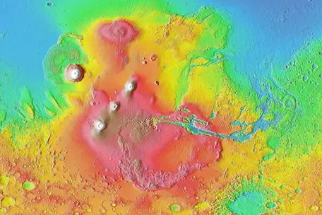 ×
MOLA shaded relief map of the Tharsis province and Valles Marineris.
×
MOLA shaded relief map of the Tharsis province and Valles Marineris.![[creative commons]](/images/creativecommons_16.png)
In-Class Activity 2
Remote Sensing_MFE
MOLA Simulation*
Purpose:
Recognize how we know about the surface of Mars using remote sensing techniques.
Preparation:
This experiment requires some space (like a hallway, or space near a cleared wall in a classroom) and will take some prep time ~ 15 mins., and ~ 20-30 mins. for students to perform the exercise. Some of the data plotting can be done as homework.
Materials Needed:
Masking tape, meter sticks or measuring tape, ping pong balls, stopwatch or watch timer, bricks or blocks that allow ping pong balls to bounce (textbooks are ineffective)
Engage
How do we know what the surface of Mars is like, especially for areas that we have only seen from a distance? Think about how dolphins know the difference between a BB gun pellet and a kernel of corn from 50' (or 16 m away). Could a similar type of detection be used to decipher the surface of Mars?
Ref. http://science.howstuffworks.com/zoology/marine-life/dolphin-disarm-sea-mine1.htm
Explore
Perform a ping-pong experiment.
Procedure:
You must have at least 2 people in your group, 3 is advisable.
Step 1:
1. Place 2 strips of tape on the wall, one approximately 2 meters (200 cm) high and the other 45 cm high and both should be at least 200 cm long and parallel; you will be using these as the points to start and stop the stopwatch.
2. One partner should hold the ping-pong ball next to the higher piece of tape, between the first finger and thumb, and approximately one inch from the wall.
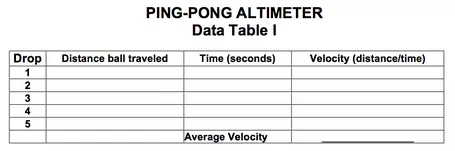
3. One partner, the "timer", should have a stopwatch and have his/her eyes level with the second piece of tape. A third partner, if available should record the results of each ball drop using the attached data sheet or one that your group makes up for itself. * Note: Use a spreadsheet for recording and calculating the data.
4. Drop the ball, and as you do say, "Go." The timer starts the stopwatch on "Go."
5. The timer will stop the watch when the ball rebounds and reaches the lower line, i.e. the clock starts when the ball drops and stops when the ball reaches the second piece of tape. Record the time on the data sheet. Repeat this step four more times.
6. Calculate the velocities (V=D/T). The distance (D) is the combination of the height of the high tape plus the height of the low tape. After finding the velocity for each of the trials, find the average velocity of the ping-pong ball. This average will be used later in this lab. It will be your baseline for comparing data.
Step 2:
Now that you have found the velocity of the ping-pong ball, you will use this information to plot the topography along a line of latitude of an asteroid. You will be creating your own asteroid terrain on the floor against the wall where you just did Step One.
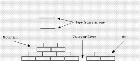
1. Create the topography model of your asteroid, along the wall where you did Step One. In order to do this you need to place wooden blocks against the wall in a line about 6-8 feet long. Be sure that you build in some hills, mountains, valleys, etc. (See Figure below)
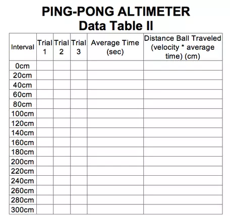
2. Starting at the beginning of the top piece of tape, place a mark every 20cm. The bottom piece does not need to be marked.
3. Again, starting at the 20cm mark you made at the beginning of the tape, you will drop the ping-pong ball as you did in Step One, and record the time in Data Table II. Drop the ball every 20cm along the tape until you reach the end. Be sure to be as accurate as you can with the timing.
4. Find the average time for each of the intervals and record it on the data table.
5. Next fill in the distance traveled in table 2 by multiplying the average velocity from table 1 by the average time just calculated at each interval.
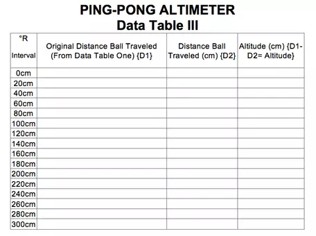
6. In data table 3, take the original distance traveled (height of high tape plus height of low tape, which will be the same for every interval) and fill in the first column of the table.
7. In the second column, take the distance ball traveled column in table 2 (last column on right) and copy that info to the 2nd column of table 3. Now, for the last column, simply subtract the 1st column data from the 2nd column data (the difference between the two) to determine the altitude of your modeled topography.
Explain
Students can explain their findings by plotting up data.
Step 3: Plotting and Graphing the Data
You will now plot the data for the average times and create graphs of the altimetry readings for your topographic model. The graphs will use different intervals between readings, so that you can compare the preciseness of different levels of accuracy (called spatial resolution).
Graph 1
1. Plot the average time for every 60cm interval. (0cm, 60cm, 120cm, etc. with time on the y-axis and distance along the x-axis)
2. Connect the points with a smooth line.
3. Label the graph appropriately.
Graph 2
1. Plot the average time for every 40cm interval. (0cm, 40cm, 80cm, etc. with time on the y-axis and distance on the x-axis)
2. Connect the points with a smooth line.
3. Label the graph appropriately.
Graph 3
1. Plot the average time for every 20cm interval. (0cm, 20cm, 40cm, 60cm, etc. with time on the y-axis and distance on the x-axis).
2. Connect the points with a smooth line.
3. Label the graph appropriately.
Elaborate
Follow-Up Questions:
1. Why is it important to keep the distance between each altimeter measurement consistent?
2. How could we make the topographical profile more accurate?
3. What does the graph look like in the comparison to your model (i.e. the same, inverted etc.)?
4. Which looks more like the model, the graph you generated from the shorter or longer distance between readings (intervals)? Why is this?
Evaluate
Step 4—expand your thought process:
The Laser Rangefinder aboard NEAR sends out a laser beam and "catches" it as it returns from being reflected by the surface of 433 Eros. The instrument records how long it takes the beam to reach the surface and bounce back up. The scientists know how fast the beam is traveling; therefore, they can calculate how far it traveled. By measuring this time and multiplying by the velocity of the beam, they calculate how far the laser has traveled. They must then divide the distance the beam traveled in half.
1. Why did you not divide in half to find the distance to the object in your topography model?
Next, the scientist must compare this distance to a "baseline" distance we will call zero. On Earth, we might use sea level as the baseline. Another way to set the baselines is to start at the center of the planetary body being studied and draw a perfect circle as close to the surface of the body as possible. Using this baseline, the altitude compared to zero can be calculated and graphed. (Here, on Earth, we often say that some point is a certain number of feet above of below sea level.)
1. Why do we not use the term "Sea level" for Mars and other planets?
2. You will now calculate the altitude of the points along your model. To do this subtract the distance the ball traveled, at each interval (from Data Table II) from the distance the ball traveled in Step One (column B, Data Table I). The number you come up with will be zero or greater. Use Data Table III to do your calculations. {The number in column B in this table should be the same for every interval. Remember, it was the baseline altitude and does not change.}
*This exercise was adapted from: Goddard Space Flight Center: https://attic.gsfc.nasa.gov/mola/pingpong.html